Searching for Fixed-Radius Near Neighbors with Cell Lists Algorithm in Julia Language

Jaan Tollander de Balsch

Last updated on 2021-03-11 Algorithms

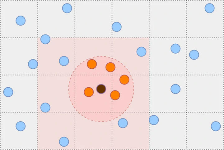
Table of Contents

Introduction

This article defines the fixed-radius near neighbors search problem and why efficient algorithms are essential. We present two algorithms for solving the problem, Brute Force and Cell Lists. We explain both algorithms in-depth and analyze their performance. We accompanied this article with a Julia implementation of the Cell Lists algorithm, located in CellLists.jl repository. We can use the algorithm in a simulation or as a reference for implementing it in another language. Cell Lists is applicable in simulations with finite range interaction potentials where we are required to compute all close pairs in each time step, such as particle simulations. For long-range interaction potentials, we recommend reading about Barnes-Hut simulation and Fast multipole method.

Fixed-radius near neighbors is an old computer science problem closely related to sorting. We define the problem as finding all pairs of points within a certain distance apart, referred to as all close pairs. The author of ¹ has surveyed different methods for solving the fixed-radius near neighbors problem. These methods include brute force, projection that is, dimension-wise sorting and querying using binary search, cell techniques, and k-d trees. The paper ² analyzes the brute force, projection, and cell techniques. In the context of particle simulations, ³ discusses Verlet Lists, a method with similarities to Cell Lists. These methods have also been applied to large scale particle simulations using GPU by ⁴.

Similar to sorting, the computational complexities of the different methods in respect to the number of particles $n$ are $O (n^{2})$ for the Brute Force approach, $O (n \log n)$ for comparison sort based approaches such as projection and k-d trees, and $O (n)$ for bucket sort based approaches such as cell techniques. However, the $O$ -notation hides the constant that depends exponentially on the dimension $d$ for comparison and bucket-based approaches. Nevertheless, in low dimensional spaces, these methods can be significantly more efficient than the Brute Force.

Regarding analyzing algorithms, we recommend Introduction to Algorithms ⁵ textbook. Foundations, sorting, hash tables, and computational geometry sections are relevant to this article. The computational geometry section contains a chapter (33.4) about finding the closest pair of points in two dimensions, which is related to finding all close pairs.

Fixed-Radius Near Neighbors Problem

Let $I = {1, \dots, n}$ denote the indices of $n \in ℕ$ points, $r > 0$ denote a fixed radius, and $𝐩_{i} \in ℝ^{d}$ denote the coordinates of the point $i \in I$ in $d \in ℕ$ dimensional Euclidean space and norm as $‖ \cdot ‖$ . The near neighbors of point $i$ are the distinct points $j \in I, j \neq i$ within radius $r,$ denoted as

\begin{matrix} (1) & N_{r} (i) = {j \in I ∣ j \neq i, ‖ 𝐩_{i} - 𝐩_{j} ‖ \leq r} . \end{matrix}

Using the definition of near neighbors, we define all close pairs as

\begin{matrix} (2) & \begin{aligned} N_{r} & = {(i, j) ∣ i \in I, j \in N_{r} (i)} \\ = {(i, j) ∣ i, j \in I, i \neq j, ‖ 𝐩_{i} - 𝐩_{j} ‖ \leq r} . \end{aligned} \end{matrix}

Because the norm is symmetric, that is $‖ 𝐩_{i} - 𝐩_{j} ‖ = ‖ 𝐩_{j} - 𝐩_{i} ‖,$ the order of $i$ and $j$ does not matter. We can simplify the all close pairs to symmetric all close pairs where we use the set ${i, j}$ to denote the inclusion of either $(i, j)$ or $(j, i),$ defined as

\begin{matrix} (3) & {\hat{N}}_{r} = {{i, j} ∣ i, j \in I, i \neq j, ‖ 𝐩_{i} - 𝐩_{j} ‖ \leq r} . \end{matrix}

The next sections discuss how to implement algorithms for fixed-radius near neighbors search.

Brute Force Algorithm

The Brute Force is the simplest algorithm for computing the near neighbors. It serves as a benchmark and building block for the Cell Lists algorithm, and it is useful for testing the correctness of more complex algorithms.

The Brute Force algorithm directly follows the definition symmetric all close pairs. It iterates over the points pairs, checks the distance condition, and yields all pairs that satisfy the condition. The following Julia code demonstrates the Brute Force approach.

@inline function distance_condition(p1::Vector{T}, p2::Vector{T}, r::T) where T <: AbstractFloat
    sum(@. (p1 - p2)^2) ≤ r^2
end

function brute_force(p::Array{T, 2}, r::T) where T <: AbstractFloat
    ps = Vector{Tuple{Int, Int}}()
    n, d = size(p)
    for i in 1:(n-1)
        for j in (i+1):n
            if @inbounds distance_condition(p[i, :], p[j, :], r)
                push!(ps, (i, j))
            end
        end
    end
    return ps
end

n, d = 10, 2
r = 0.1
p = rand(n, d)
brute_force(p, r)

The Brute Force algorithm performs a total number of iterations:

$\begin{matrix} (4) & B (n) = \sum_{i = 1}^{n - 1} i = \frac{n (n - 1)}{2} \in O (n^{2}) . \end{matrix}$

Since Brute Force has quadratic complexity, it does not scale well for many points, motivating the search of more efficient algorithms.

Cell Lists Algorithm

Definition

The Cell Lists algorithm works by partitioning the space into a grid with cell size $r$ and then associates each cell to the points that belong to it. The partitioning guarantees that all points within distance $r$ are inside a cell or its neighboring cells. We refer to the set of all such point pairs as cell list pairs $C .$ It contains all close pairs by the relation ${\hat{N}}_{r} \subseteq C \subseteq {\hat{N}}_{R},$ where $R = 2 r \sqrt{d}$ is the maximum distance between two points in neighboring cells. Therefore, we can find all close pairs by iterating over cell list pairs and checking the distance condition.

The Julia code is available as a GitHub repository at CellLists.jl.

We implement the Cell Lists algorithm in Julia language. The algorithm has two parts. The first one constructs the Cell List, and the second one iterates over it to produce the symmetric all close pairs.

Constructor

The CellList constructor maps each cell to the indices of points in that cell.

struct CellList{d}
    indices::Dict{CartesianIndex{d}, Vector{Int}}
end

function CellList(p::Array{T, 2}, r::T, offset::Int=0) where T <: AbstractFloat
    @assert r > 0
    n, d = size(p)
    cells = @. Int(fld(p, r))
    data = Dict{CartesianIndex{d}, Vector{Int}}()
    for j in 1:n
        @inbounds cell = CartesianIndex(cells[j, :]...)
        if haskey(data, cell)
            @inbounds push!(data[cell], j + offset)
        else
            data[cell] = [j + offset]
        end
    end
    CellList{d}(data)
end

Near Neighbors

We define the indices to the neighboring cells as follows:

@inline function neighbors(d::Int)
    n = CartesianIndices((fill(-1:1, d)...,))
    return n[1:fld(length(n), 2)]
end

We only include half of the neighboring cells to avoid double counting when iterating over the neighboring cells of all non-empty cells. We also define functions for brute-forcing over a set of points.

@inline function distance_condition(p1::Vector{T}, p2::Vector{T}, r::T) where T <: AbstractFloat
    sum(@. (p1 - p2)^2) ≤ r^2
end

@inline function brute_force!(ps::Vector{Tuple{Int, Int}}, is::Vector{Int}, p::Array{T, 2}, r::T) where T <: AbstractFloat
    for (k, i) in enumerate(is[1:(end-1)])
        for j in is[(k+1):end]
            if @inbounds distance_condition(p[i, :], p[j, :], r)
                push!(ps, (i, j))
            end
        end
    end
end

@inline function brute_force!(ps::Vector{Tuple{Int, Int}}, is::Vector{Int}, js::Vector{Int}, p::Array{T, 2}, r::T) where T <: AbstractFloat
    for i in is
        for j in js
            if @inbounds distance_condition(p[i, :], p[j, :], r)
                push!(ps, (i, j))
            end
        end
    end
end

Finding all cell list pairs works by iterating over all non-empty cells and finding the pairs within that cell using Brute Force. Iterating over its neighboring cells checks if the cell is non-empty and finds the pairs between the current and the non-empty neighboring cell using Brute Force.

function near_neighbors(c::CellList{d}, p::Array{T, 2}, r::T) where d where T <: AbstractFloat
    ps = Vector{Tuple{Int, Int}}()
    offsets = neighbors(d)
    # Iterate over non-empty cells
    for (cell, is) in c.data
        # Pairs of points within the cell
        brute_force!(ps, is, p, r)
        # Pairs of points with non-empty neighboring cells
        for offset in offsets
            neigh_cell = cell + offset
            if haskey(c.data, neigh_cell)
                @inbounds js = c.data[neigh_cell]
                brute_force!(ps, is, js, p, r)
            end
        end
    end
    return ps
end

Usage

We can use the Cell Lists by first constructing the CellList and then query the symmetric all close pairs with near_neighbors.

n, d = 10, 2
r = 0.1
p = rand(n, d)
c = CellList(p, r)
indices = near_neighbors(c, p, r)

We receive the same output as for brute force.

indices2 = brute_force(p, r)
@assert Set(Set.(indices)) == Set(Set.(indices2))

In the next section, we analyze the Cell Lists algorithm’s performance compared to Brute Force and theoretical limits and discuss the assumptions when Cell Lists is practical.

Analysis

Number of Iterations

We denote the number of non-empty cells using

\begin{matrix} (5) & \hat{n} \in {1, 2, . . ., n} . \end{matrix}

Each non-empty cell has $n_{1}, n_{2}, \dots, n_{\hat{n}}$ points such that that the total number of points is $n = n_{1} + n_{2} + \dots + n_{\hat{n}} .$ Then, the number of iterations to find cell list pairs is

M (\hat{n}) = \sum_{i = 1}^{\hat{n}} (B (n_{i}) + \sum_{j \in N (i)} n_{i} \cdot n_{j})

\begin{matrix} (6) & = \sum_{i = 1}^{\hat{n}} B (n_{i}) + \sum_{i = 1}^{\hat{n} - 1} \sum_{j \in N (i)} n_{i} \cdot n_{j} \end{matrix}

where $N (i)$ is half of the non-empty neighboring cells of cell $i$ where $N (\hat{n}) = \emptyset .$ We can iterate over the neighboring cell pairs (highlighted in red) in two ways.

Method 1: For each non-empty cell $i \in {1, \dots, \hat{n} - 1},$ iterate over the remaining non-empty cells $j = {i, \dots, \hat{n}}$ and check if they are a neighbor, which takes $B (\hat{n})$ iterations.

Method 2: For each non-empty cell $i \in {1, \dots, \hat{n} - 1},$ iterate over neighboring cells and check if they are non-empty (as in near_neighbors code), which takes $\hat{n} \cdot m_{d}$ iterations where $m_{d} = (3^{d} - 1) / 2$ is the number of neighboring cells in dimension $d .$

We derive the dimensionality condition such that method 2 performs fewer iterations compared to method 1:

\begin{matrix} (7) & \begin{aligned} \hat{n} \cdot m_{d} & < B (\hat{n}) \\ \hat{n} & > 3^{d}, \end{aligned} \end{matrix}

When true, finding neighboring cells grows linearly, necessary for the Cell Lists to be efficient compared to Brute Force. Note that higher-dimensional spaces require exponentially higher numbers of non-empty cells $\hat{n}$ to satisfy the condition.

Worst-Case Instances

If one cell contains all the points, we have $\hat{n} = 1,$ and $n_{1} = n,$ the number of iterations equal to Brute Force

$\begin{matrix} (8) & M (1) = B (n_{1}) + 0 = B (n) . \end{matrix}$

If all points are in unique cells and we do not satisfy the dimensionality condition, we have $\hat{n} = n$ and $n_{1}, n_{2}, \dots n_{\hat{n}} = 1$ and $\hat{n} \leq 3^{d},$ the number of iterations equals to Brute Force

$\begin{matrix} (9) & M (n) = \hat{n} + B (\hat{n}) = B (n) + n . \end{matrix}$

Curse of Dimensionality

Cell Lists also suffers from the curse of dimensionality. As we increase the dimension, the number of possible cells grows exponentially. That is,

$\begin{matrix} (10) & \prod_{i = 1}^{d} (\frac{l_{i}}{r}) \geq {(\frac{l}{r})}^{d}, \end{matrix}$

where $l_{1}, l_{2}, \dots, l_{d}$ are the lengths of the minimum bounding box and $min {l_{1}, l_{2}, \dots, l_{d}} = l > r$ is the minimum length. Therefore, if we draw two random cells from a non-exponential probability distribution where possible cells are its states, the probability that they are the same cell decreases exponentially as the dimension grows. Consequently, the number of non-empty cells approaches the number of points $\hat{n} \to n,$ and the dimensionality condition requires larger $\hat{n}$ to satisfy. Thus the performance approaches the worst-case.

Practical Instances

In many practical instances, we can assume a limit to how many points can occupy a cell. For example, two and three-dimensional physical simulations particles have finite size and non-overlapping and satisfy the dimensionality condition.

For a problem instance that satisfies the dimensionality condition $\hat{n} > 3^{d},$ and the number of points per cell is limited by $1 \leq n_{1}, n_{2}, \dots, n_{\hat{n}} \leq \bar{n}$ where $\bar{n}$ is independent of $n .$ By assuming that every cell is filled $n_{1}, n_{2}, \dots, n_{\hat{n}} = \bar{n}$ , we have $n = \hat{n} \cdot \bar{n}$ , and we obtain an upper bound for the number of iterations

\begin{matrix} (11) & M (\hat{n}) \leq \hat{n} \cdot B (\bar{n}) + \hat{n} \cdot m_{d} \cdot {\bar{n}}^{2} \leq (m_{d} + 1) \cdot \bar{n} \cdot n \end{matrix}

With fixed dimension and maximum density, the number of iterations is linearly proportional to the number of points $O (n)$ . The constant term can be large; therefore, we should always measure the Cell Lists’ performance against the Brute Force on real machines with realistic problem instances.

Benchmarks

Method

We performed each benchmark instance by setting fixed parameter values for size $n$ , dimension $d$ , and radius $r,$ and generating $n$ points $𝐩 = (p_{1}, \dots, p_{d})$ where we draw the coordinate values from a uniform distribution, that is, $p_{i} \sim U (0, 1)$ for all $i = 1, \dots, d .$ We measured the performance of each instance using BenchmarkTools.jl and selected the median time. We performed the benchmarks on the Aalto Triton cluster running on Intel(R) Xeon(R) CPU E5-2680 v4 @ 2.40GHz processors.

You can find the benchmarking code from the CellListsBenchmarks.jl GitHub repository and the scripts to run the benchmarks and plotting from cell-lists-benchmarks GitHub repository.

Cell Lists vs. Brute Force

Time in microseconds as a function of number of points $n$ for dimension $d=2$ and radius $r=0.01$. — Time in microseconds as a function of number of points $n$ for dimension $d = 2$ and radius $r = 0.01$ .

Time in microseconds as a function of number of points $n$ for dimension $d=3$ and radius $r=0.01$. — Time in microseconds as a function of number of points $n$ for dimension $d = 3$ and radius $r = 0.01$ .

Time in microseconds as a function of number of points $n$ for dimension $d=4$ and radius $r=0.01$. — Time in microseconds as a function of number of points $n$ for dimension $d = 4$ and radius $r = 0.01$ .

Time in microseconds as a function of number of points $n$ for dimension $d=5$ and radius $r=0.01$. — Time in microseconds as a function of number of points $n$ for dimension $d = 5$ and radius $r = 0.01$ .

The figures above show how Cell Lists compares to Brute Force as we increase dimension with a constant radius. As can be seen, Cell Lists performs better in low dimensions and beat Brute Force with a small number of points, but requires more points with a larger dimension.

Effects of Dimensionality

Time in microseconds as a function of number of points $n$ for dimensions $d=2,...,5$ and radius $r=0.01$. — Time in microseconds as a function of number of points $n$ for dimensions $d = 2, \dots, 5$ and radius $r = 0.01$ .

The ratio to $d=2$ results as a function of number of points $n$ for dimensions $d=2,...,5$ and radius $r=0.01$. — The ratio to $d = 2$ results as a function of number of points $n$ for dimensions $d = 2, \dots, 5$ and radius $r = 0.01$ .

The figure above shows the relation between Cell Lists with increasing dimension and constant radius. As we can see, the increase in time scales roughly to $3^{d} .$

Conclusions

I first encountered the fixed-radius near neighbors problem while developing the Crowd Dynamics simulation, which is mechanistically similar to molecular simulation with finite distance interactions (local interactions). The algorithms presented in this article can be used for research purposes or building small scale simulations. Large scale simulations may require additional improvements such as parallelism, which we discuss more in Multithreading in Julia Language Applied to Cell Lists Algorithm.

Contribute

If you enjoyed or found benefit from this article, it would help me share it with other people who might be interested. If you have feedback, questions, or ideas related to the article, you can contact me via email. For more content, you can follow me on YouTube or join my newsletter. Creating content takes time and effort, so consider supporting me with a one-time donation.

References

Bentley, J. L. (1975). A Survey of techniques for fixed radius near neighbor searching, 37. ↩︎
Mount, D. (2005). Geometric Basics and Fixed-Radius Near Neighbors, 1–8. ↩︎
Yao, Z., Wang, J. S., Liu, G. R., & Cheng, M. (2004). Improved neighbor list algorithm in molecular simulations using cell decomposition and data sorting method. Computer Physics Communications, 161(1–2), 27–35. https://doi.org/10.1016/j.cpc.2004.04.004 ↩︎
Hoetzlein, R. (2014). Fast Fixed-Radius Nearest Neighbors: Interactive Million-Particle Fluids. GPU Technology Conference. ↩︎
Cormen, T. H., Leiserson, C. E., Rivest, R. L., & Stein, C. (2009). Introduction to Algorithms, Third Edition (3rd ed.). The MIT Press. ↩︎

Cell Lists Fixed-Radius Near Neighbors Search Julia Language