Multithreading in Julia Language Applied to Cell Lists Algorithm
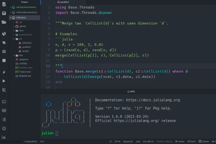
Table of Contents
Introduction
In the past, the serial performance of processors increased by Moore’s law, and personal computers relied on it for their single-core performance. Only the most powerful supercomputer had multiple cores to perform multiple operations at once. However, times have changed, and the single-core processor performance no longer increases by Moore’s law. Hence manufacturers began adding more cores to processors, and programmers must adapt to these changes by developing their algorithms to effectively use multiple cores if they wish to increase the performance of their code.
An algorithm that uses only a single core is referred to as a serial algorithm and performs one operation at a time. By parallelizing a serial algorithm, we convert it to a parallel algorithm that performs multiple operations simultaneously. Parallel programming represents a new programming paradigm with unique challenges compared to serial programming and requires programmers to learn the principles of this new paradigm.
This article teaches you how to use multithreading in Julia Language to parallelize serial algorithms. As a practical example, we explore how to convert the serial Cell Lists algorithm from the article Searching for Fixed-Radius Near Neighbors with Cell Lists Algorithm in Julia Language into a multithreaded version. We recommend reading it before the Multithreaded Cell Lists Algorithm section.
Multithreading
Task Parallelism
The Julia language implements multithreading using task parallelism where tasks communicate in shared memory as described in their article Announcing composable multi-threaded parallelism in Julia.
In task parallelism, a task refers to a computational task such as executing a function. The workload of a task measures how much work is required to compute it. We refer to creating a new task as spawning a task. By spawning multiple tasks we form a pool of tasks.
Composable task parallelism means that a task can spawn new tasks. Composability makes task parallelism more dynamic for workloads that are unknown before execution as they would often lead to unevenly balanced resource utilization. We can think of the execution of tasks as a tree, where each task represents a node that has edges to the tasks it spawned.
In task parallelism, a scheduler assigns tasks from the pool to multiple threads that run simultaneously. A static scheduler pre-assigns all tasks to run on specific threads. On the other hand, a dynamic scheduler assigns a new task to a thread from the pool when a previous task has finished. Schedulers can use different policies for the order in which they assign new tasks to threads, which has a large effect on the performance of multithreading. The Julia’s multithreading uses a dynamic scheduler based on depth-first scheduling.
Parallelizability
We can think parallelizing algorithms in three steps: divide, conquer, and combine. First, we divide a task it into independent subtasks whose workloads are as evenly distributed as possible. Each subtask computes a part of the original task. In the conquer step, we compute subtasks independently in parallel. Finally, we combine the results from subtasks into a result for the original task. Composability gives us the ability to use these steps recursively on the conquer step by further diving a subtask into its subtasks, and then conquering and combining them.
When dividing a task into subtasks with even workloads is trivial, we refer to the algorithm as perfectly parallel and typically use static scheduling. If it is not possible to divide a task into independent subtasks, we say that the algorithm is unparallelizable. The difficulty of dividing a task into subtasks depends on its properties.
Tasks on different threads should not write data to the same memory locations to avoid data races. If they do, they have use a lock or atomic operations to avoid other threads writing data to the memory location at the same time.
The goal of developing a parallel algorithm is to create a correct algorithm that achieves a large enough proportional speedup to the number of threads to justify the increased resource usage. We should always develop a serial algorithm before the parallel algorithm. The speedup is affected by the task size, the number of threads, the overhead of dividing, combining and scheduling tasks, and the workload of each subtask. An efficient parallel algorithm aims to balance the total workload between threads.
The serial algorithm works as a building block for the parallel algorithm. Also, we can compare the output and benchmark the parallel implementation against the serial implementation to catch errors and measure the speedup on real machines. Verifying the correctness of a parallel algorithm, such as proving race conditions do not occur, requires analyzing it using formal methods. However, we can avoid most race conditions by using high-level constructs and following established design patterns for implementing parallelism.
Running Julia with Multiple Threads
We need to set the number of threads when starting Julia. In Julia version 1.5 and above, we can use the -t/--threads argument.
julia --threads 4
If we are using Julia version from 1.3 to 1.4, we have to set the JULIA_NUM_THREADS environment variable before executing Julia to use multiple threads.
export JULIA_NUM_THREADS=4
We can import the multithreading library from Base.
using Base.Threads
We can query the available threads using nthreads function.
nthreads()
Typically, we use the number of threads when allocating thread-specific memory locations (in shared memory) for writing data to avoid race conditions. We can also query the thread ID, an integer between 1 and nthreads(), using the threadid function.
threadid()
We can use thread ID in indexing when accessing the thread-specific memory locations for writing data.
We recommend watching the Multi-Threading Using Julia for Enterprises webinar recording by Julia Computing, which shows how to apply multithreading in practice.
Static Scheduling
If we can easily compute the exact workload of subtasks before execution, we can use static scheduling, which divides the workloads evenly for each available thread. Formally, dividing the subtasks is an optimization problem where we aim to minimize the maximum workload. We may have to use heuristics if solving the exact value of the optimization problem is too difficult.
In Julia language, we can use the @threads macro for static scheduling of for-loops. It splits the iterations evenly among available threads. For example, we can sum an array of random numbers in parallel using static schedculing.
a = rand(100000)  # Create array of random numbers
p = zeros(nthreads())  # Allocate a partial sum for each thread
# Threads macro splits the iterations of array `a` evenly among threads
@threads for x in a
   p[threadid()] += x  # Compute partial sums for each thread
end
s = sum(p)  # Compute the total sum
Note how we use nthreads and threadid to ensure that each threads writes data to thread-specific memory location to avoid data race.
Dynamic Scheduling
We cannot always compute the exact workload of subtasks before execution. In this case, we want to create many subtasks and assign them to threads using dynamic scheduling. We should create subtasks such that we estimate that the workload is not so small that threading overhead becomes significant and not so large so that scheduler cannot balance the workload. Because subtasks vary in workload, each thread may execute a different number of subtasks.
In Julia language, the Task datatype represents a task. We can use the @spawn and @sync macros to schedule tasks dynamically and the fetch function to retrieve the output value of the task. The @spawn macro creates new tasks for the scheduler. The @sync macro synchronizes the tasks in its scope. It means that code written after the scope of @sync executes once all tasks inside its scope have finished. Since Julia’s multithreading is composable, we can call spawn and sync macros inside other tasks. We need to explicitly import the spawn macro from Base.Threads.
using Base.Threads: @spawn
As an example of dynamic scheduling, we define a task with a variable workload. The task then returns the workload.
function task()
    x = rand(0.001:0.001:0.05)  # Generate a variable workload
    sleep(x)  # Sleep simulates the workload
    return x  # Return the workload
end
Next, we spawn n tasks to that are dynamically scheduled to execute on available threads and we accumulate the total workloads per thread.
n = 1000  # Number of tasks
p = zeros(nthreads())  # Total workload per thread
@sync for i in 1:n
   @spawn p[threadid()] += task()  # Spawn tasks and sum the workload
end
We can compute how well the workloads are balanced by computing the ratio of workload per thread to the total workload.
julia> s = sum(p)  # Total workload
julia> println(round.(p/s, digits=3))
[0.251, 0.251, 0.251, 0.246]
We will obtain quite evenly balanced ratios when n is large enough.
Measuring Performance
We use the same performance measures for multithreaded algorithms as the multithreading chapter in Introduction to Algorithms book 1. The book defines the running time $T_P$ of multithreaded computation using $P$ threads, work $T_1$ as the time to execute all tasks using a single thread, and span $T_∞$ as the time of the longest-running strand of computation. Speedup $T_1/T_P$ of a multithreaded algorithm tells how many times faster the computation is on $P$ threads than a single thread. Parallelism $T_1/T_∞$ gives an upper bound to the possible speedup $$T_1/T_P≤T_1/T_∞ < P.$$
We can experimentally measure the speedup of the parallel algorithm against the serial algorithm and determine a threshold for the input size where the speedup is larger than one, $T_1/T_P>1.$ That is, the parallel algorithm is faster than the serial one.
Multithreaded Cell Lists Algorithm
Introduction
You can find all Julia code from the CellLists.jl GitHub repository.
This section extends the serial Cell Lists algorithm into a multithreaded version using the divide, conquer, and combine steps. In these steps, we divide input into multiple tasks, conquer tasks by scheduling tasks on available threads, and combine subtask results by reducing them with a binary operation.
We will use CellList, neighbors, and brute_force! from the serial Cell Lists algorithm. The CellList constructor is perfectly parallel because the input is easy to divide into near equal-sized subtasks. However, efficiently parallelizing the near_neighbors function is more challenging because the subtask workload varies.
Multithreaded Constructor
using Base.Threads

function Base.merge(c1::CellList{d}, c2::CellList{d}) where d
    CellList{d}(merge(vcat, c1.data, c2.data))
end

function CellList(p::Array{T, 2}, r::T, ::Val{:threads}) where T <: AbstractFloat
    t = nthreads()
    n, d = size(p)
    # Divide
    cs = cumsum(fill(fld(n, t), t-1))
    parts = zip([0; cs], [cs; n])
    # Conquer
    results = Array{CellList{d}, 1}(undef, t)
    @threads for (i, (a, b)) in collect(enumerate(parts))
        results[i] = CellList(p[(a+1):b, :], r, a)
    end
    # Combine
    return reduce(merge, results)
end
The multithreaded CellList constructor divides the points p into equal-sized parts, then spawns a thread for each part and constructs the CellList for that part. Finally, it merges the resulting CellLists into one.
Multithreaded Near Neighbors
function brute_force_cell!(pts, cell, is, p, r, data, offsets)
    # Pairs of points within the cell
    brute_force!(pts[threadid()], is, p, r)
    # Pairs of points with non-empty neighboring cells
    for offset in offsets
        neigh_cell = cell + offset
        if haskey(data, neigh_cell)
            @inbounds js = data[neigh_cell]
            brute_force!(pts[threadid()], is, js, p, r)
        end
    end
end

function near_neighbors(c::CellList{d}, p::Array{T, 2}, r::T, ::Val{:threads}) where d where T <: AbstractFloat
    offsets = neighbors(d)
    pts = [Vector{Tuple{Int, Int}}() for _ in 1:nthreads()]
    data = collect(c.data)
    perm = sortperm(@. length(getfield(data, 2)))
    # Iterate over non-empty cells in decreasing order of points per cell
    @sync for (cell, is) in reverse(data[perm])
        @spawn brute_force_cell!(pts, cell, is, p, r, c.data, offsets)
    end
    return reduce(vcat, pts)
end
The parallel Near Neighbors method creates a new task for iterating over near neighbors of each non-empty cell. Creating multiple tasks allows the algorithm to benefit from the dynamic scheduling since the workload of each task may vary depending on how many points the cell and its neighbors contain. We estimate the workload of tasks by the number of points in the cell. Therefore, we spawn the task in descending order of the estimated workload so that longer tasks are spawned before shorter ones. After the tasks have finished, the algorithm concatenates the resulting arrays of point pairs into the final result.
Usage
We can use the multithreaded algorithms for Cell Lists by dispatching the CellList constructor and near_neighbors function with the Val(:threads) value type.
n, d = 20000, 2
r = 0.01
p = rand(n, d)
c = CellList(p, r, Val(:threads))
indices = near_neighbors(c, p, r, Val(:threads))
Furthermore, we can iterate over the resulting indices using multithreading. For example, we could use static scheduling with @threads since the workload for each pair of indices is usually identical.
@threads for (i, j) in indices
    # perform computations on near neighbors p[i, :] and p[j, :]
end
Benchmarks
Method
We performed each benchmark instance by setting fixed parameter values for size $n$, dimension $d$, and radius $r,$ and generating $n$ points $𝐩=(p_1,…,p_d)$ where we draw the coordinate values from a uniform distribution, that is, $p_i∼U(0, 1)$ for all $i=1,…,d.$ We measured the performance of each instance using BenchmarkTools.jl and selected the median time. We performed the benchmarks on the Aalto Triton cluster running on Intel(R) Xeon(R) CPU E5-2680 v4 @ 2.40GHz processors.
You can find the benchmarking code from the CellListsBenchmarks.jl GitHub repository and the scripts to run the benchmarks and plotting from cell-lists-benchmarks GitHub repository.
Serial vs. Multithreaded Constructor


As we can see, multithreading significantly speeds up the Cell Lists construction. Dimensionality does not have a significant effect on the construction time.
Serial vs. Multithreaded Near Neighbors


We subtracted the time spent in garbage collection from the measurements. We can see that with $4$ threads, the mean parallel speedup is close to $2$ for the particular instance. The serial times seem to vary between instances, which is most likely an artifact from the benchmarking that we have to resolve in the future.
In general, we need to benchmark the parallel near neighbors with our target parameter values to know whether the performance of the parallel version is better than the serial version.
Conclusion
By now you have learned the basics of task-based parallelism and can start developing multithreaded algorithms using the Julia language. We have also seen how applying multithreading to the Cell Lists algorithm obtained a generous speedup compared to the serial algorithm. For further exploration, you may want to look up the ThreadsX library, which implements parallel versions of many Base functions.
Contribute
If you enjoyed or found benefit from this article, it would help me share it with other people who might be interested. If you have feedback, questions, or ideas related to the article, you can contact me via email. For more content, you can follow me on YouTube or join my newsletter. Creating content takes time and effort, so consider supporting me with a one-time donation.
References
Cormen, T. H., Leiserson, C. E., Rivest, R. L., & Stein, C. (2009). Introduction to Algorithms, Third Edition (3rd ed.). The MIT Press. ↩︎
Jaan Tollander de Balsch
Jaan Tollander de Balsch is a computational scientist with a background in computer science and applied mathematics.