Measuring Tail Risk Using Conditional Value at Risk
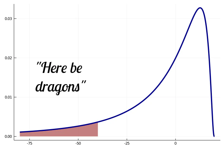
Table of Contents
Introduction
This article explores how to measure the risk of processes that involve uncertainty. We find these processes from fields such as finance, economics, and biology in real life. We will use analogies form these fields to explain the concepts related to risk and uncertainty. We refer to negative outcomes as downside or cost and positive outcomes as upside or profit.
First, we need to distinguish the difference between small and large risks. We can think of small risks as operational costs resulting in lost resources, such as time, money, and effort in amounts that can be justified by the potential profits and do not threaten existence. For example, a business can spend time and money to test new product designs. The designs may increase sales and result in profits or fail, and result in losses.
On the other hand, large risks, aka worst-case risks, include catastrophic events such as bankruptcy, injury, or death. It can be difficult or impossible to recover from a catastrophic event; hence, they may pose an existential threat to the entity. If the entity has to slow or halt its activities, it can no longer produce a positive upside, such as monetary profits. Thus, the purpose of quantifying risk is to minimize the chances of catastrophic events. However, keep in mind that models can only quantify risks it accounts for, not risks outside the model. In real-life, risks outside the model exists, and their outcomes may be significant.
The difference between what is considered small and large risks depends on the size of the entity. For example, a lawsuit might destroy a small company, but large companies often have legal teams just for handling cases, making them operational costs.
For quantifying risk, we explore a class of risk measures called coherent risk measures. They have properties that make them applicable for fields such as finance and efficient for mathematical optimization. As a concrete example of a coherent risk measure, we introduce conditional value at risk, also known as the Expected Shortfall. We recommend reading the original paper 1, which covers the formula’s full derivation, proofs, and discussion. This article aims to make it easy and fast to implement and understand Conditional Value at Risk, whereas the original article is quite laborious to understand.
Coherent Risk Measures
Consider a set $V$ of real-valued random variables. A coherent risk measure is a function $ρ:V→ℝ$ that satisfies the following properties:
Normalized. $$ρ(0)=0. \tag{1}$$ The risk of holding no assets is zero.
Monotonicity. For all $X,Y∈V, X≤Y$: $$ρ(X)≤ρ(Y). \tag{2}$$ Higher losses mean higher risk.
Subadditivity. For all $X,Y,X+Y∈V$: $$ρ(X+Y)≤ρ(X)+ρ(Y). \tag{3}$$ Diversification decreases risk.
Positive homogeneity. For all $X, h⋅X∈V, h≥0$: $$ρ(h⋅X)=h⋅ρ(X). \tag{4}$$ Risk of a position is proportional to its size.
Translation invariance. For all $X∈V, c∈ℝ$: $$ρ(X+c)=ρ(X)-c. \tag{5}$$ Adding a certain gain decreases the risk by the same amount.
A corollary from subadditivity and positive homogeneity is that a coherent risk measure $ρ$ is convex. Formally, for all $X,Y∈V, λ∈[0,1]$:
$$ρ(λ⋅X + (1-λ)⋅Y) ≤ λ⋅ρ(X) + (1-λ)⋅ρ(Y). \tag{6}$$
Convexity makes coherent risk measures efficient to solve when used in mathematical optimization.
When using risk measures, it is essential to consider whether properties support a particular process. For example, subadditivity may not hold for measuring the risk of bank mergers 2. Generally, for complex entities, an increase in size can increase internal friction, resulting in a higher risk.
Conditional Value at Risk
Prerequisites
Mathematically, we model uncertainty of a process with a probability distribution that maps different outcomes, referred to as states, to probabilities. We consider the states with negative values as risks. The left tail of a probability distribution refers to the part of the distribution with states below a certain threshold. Tail risk refers to risk measured from the left tail of the distribution.
Given a random variable $X∈V,$ we denote its domain as $x∈Ω_X,$ the probability distribution function as $f_X(x),$ the cumulative distribution function as $F_X(x),$ and the expected value as $\operatorname{E}(X).$ We define the conditional probability as $ℙ(X∣Y)=ℙ(X∩Y)/ℙ(Y)$ and an indicator function as
Definition

We define the conditional value at risk for a range of confidence levels denoted by $α∈[0, 1].$ The confidence level determines the threshold for the size of the left tail. Smaller confidence level measures a shorter left tail, excluding states with lower risk. Using the confidence level, we define the value at risk as
It is the lower bound for $x$ such that the cumulative probability is equal or above $α.$ We can also think value at risk as the generalized inverse of the cumulative distribution function. We define the conditional value at risk as an integral over the value at risk as
We have an equivalent, but more practical formulation using expected value defined as
The red part measures the expected value of the left tail distribution less or equal to the value at risk. The blue part corrects the expected value by subtracting the amount of expected value that exceeds the confidence level $α$ up to to the cumulative probability of $x_α.$ Finally, the orange part divides by the confidence level, making the value a conditional expectation of the left tail.
Limits
Conditional value at risk is a monotonically increasing function of $α$. Therefore, it has a lower bound of
and upper bound of
$$\operatorname{CVaR}_1(X) = \operatorname{E}(X). \tag{11}$$
Practical implementations of conditional value at risk omit $α=0$ from the range of confidence levels to keep the implementation simple, especially in optimization.
Continuous Case
We define the probability density function as
$$ℙ(a≤X≤b)=∫_a^b f_X(x) dx$$
such that $ℙ(-∞≤X≤∞)=1,$ and its cumulative distribution function
$$F_X(x)=∫_{-∞}^x f_X(u) du.$$
We define expected value as
$$\operatorname{E}(X)=∫_{-∞}^{∞} x f_X(x) dx.$$
The value at risk remains as
The conditional value at risk becomes
For continuous distributions, the corrective term equals zero because there are no discrete jumps. Therefore, the conditional value at risk is equivalent to the tail-conditional expected value.
Discrete Case
We define the discrete probability distribution over a domain $x∈Ω_X$ as
such that $∑_{x∈Ω_X} f_X(x)=1,$ and its cumulative distribution function as
We denote implicitly that all variables $x,x^′∈Ω_X.$ We define the expected value as
The value at risk always has a minimum. Thus we have
The conditional value at risk becomes
We can easily implement the discrete form of conditional value at risk in any programming language.
Implementation in Julia Language

The Julia code and plots are available in the ConditionalValueAtRisk GitHub repository. The example below describes the implementation and how to use it.
We can implement the value at risk and conditional value at risk functions in Julia for discrete probability distributions as follow.
"""Value at Risk."""
function value_at_risk(x::Vector{Float64}, f::Vector{Float64}, α::Float64)
    i = findfirst(p -> p≥α, cumsum(f))
    if i === nothing
        return x[end]
    else
        return x[i]
    end
end

"""Conditional Value at Risk."""
function conditional_value_at_risk(x::Vector{Float64}, f::Vector{Float64}, α::Float64)
    x_α = value_at_risk(x, f, α)
    if iszero(α)
        return x_α
    else
        tail = x .≤ x_α
        return (sum(x[tail] .* f[tail]) - (sum(f[tail]) - α) * x_α) / α
    end
end
Let us create a random discrete probability distribution.
normalize(v) = v ./ sum(v)
scale(v, low, high) = v * (high - low) + low
n = 10
x = sort(scale.(rand(n), -1.0, 1.0))
f = normalize(rand(n))
α = 0.05
Next, we assert that the inputs are valid. Note that the states $x$ do not have to be unique for the formulation to work.
@assert issorted(x)
@assert all(f .≥ 0)
@assert sum(f) ≈ 1
@assert 0 ≤ α ≤ 1
Then, executing the function in Julia REPL gives us a result.
julia> conditional_value_at_risk(x, f, α)
-0.9911100750623101
Conclusions
I became interested in risk measures from developing DecisionProgramming.jl, a Julia library for decision-making problems under uncertainty. It implements conditional value at risk as an optimization formulation used as a convex combination with the expected value. 3 Optimizing conditional value at risk is more generally discussed in 4 and 5.
Related to uncertainty and risk, I have been reading Fooled by Randomness and The Black Swan by Nassim Nicholas Taleb. These books are insightful on thinking about uncertainty and risk in real-life situations and the cognitive biases regarding how we make decisions under uncertainty. 6
Contribute
If you enjoyed or found benefit from this article, it would help me share it with other people who might be interested. If you have feedback, questions, or ideas related to the article, you can contact me via email. For more content, you can follow me on YouTube or join my newsletter. Creating content takes time and effort, so consider supporting me with a one-time donation.
References
Acerbi, C., & Tasche, D. (2002). Expected shortfall: A natural coherent alternative to value at risk. Economic Notes, 31(2), 379–388. https://doi.org/10.1111/1468-0300.00091 ↩︎
Rau-Bredow, H. (2019). Bigger is not always safer: A critical analysis of the subadditivity assumption for coherent risk measures. Risks, 7(3). https://doi.org/10.3390/risks7030091 ↩︎
Salo, A., Andelmin, J., & Oliveira, F. (2019). Decision Programming for Multi-Stage Optimization under Uncertainty. Retrieved from http://arxiv.org/abs/1910.09196 ↩︎
Rockafellar, R. T., & Uryasev, S. (1999). Optimization of Conditional Value-at-Risk, 1–26. ↩︎
Rockafellar, R. T., & Uryasev, S. (2002). Conditional value-at-risk for general loss distributions. Journal of Banking and Finance, 26(7), 1443–1471. https://doi.org/10.1016/S0378-4266(02)00271-6 ↩︎
Taleb, N. N. (2020). Statistical Consequences of Fat Tails: Real World Preasymptotics, Epistemology, and Applications. ↩︎
Jaan Tollander de Balsch
Jaan Tollander de Balsch is a computational scientist with a background in computer science and applied mathematics.