Scientific Writing with Markdown

Introduction

Markdown is a lightweight markup language with plain text formatting syntax. This article explains how to use Markdown for writing scientific, technical, and academic documents that require equations, citations, code blocks, Unicode characters, and embedded vector graphics. Markdown offers the easiest and most versatile syntax and tools for creating these types of documents.

Markdown was initially designed for creating content for websites (HTML), but we can also create other document formats such as PDF and EPUB using converters like Pandoc. We can also use Markdown to write LaTeX documents more easily compared to using pure LaTeX. Since Markdown files are text files, they need to be converted to a separate output document, unlike MS Word or Google Docs, which displays the output document while editing it. We include software recommendations for writing and converting Markdown.

To help getting started, check out the Markdown-Templates GitHub repository, which demonstrates how to create documents in practice. We explore its contents during this article.

Markdown is not the best choice for documents requiring lots of small customizations in styles, fonts, colors, or outlooks. On the other hand, Markdown excels at creating documents that need little customization or have premade styles or templates available.

Software

Converters

We need a converter to convert Markdown to other document formats. Pandoc is the primary tool that we use for converting Markdown into other formats. LaTeX is a typesetting system designed for the production of technical and scientific documentation. Pandoc requires LaTeX installation for creating PDF documents. We can install them from their respective websites, Pandoc and LaTeX.

For creating a static website to write scientific content using Markdown, we recommend using Hugo with Wowchemy. Their respective websites document them extensively, and we recommend to read them for more information.

For technical documentation, it is best to use documenting software recommended for the programming language. For example, we can use Documenter.jl to create documentation using Markdown for Julia projects.

Editors

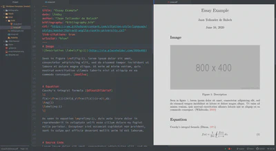
We need an editor to write Markdown effectively. The best options for writing Markdown on a desktop are Atom and Visual Studio Code. A desktop editor should have the following features:

• Support and highlighting for Markdown syntax.
• Live preview for Markdown documents.
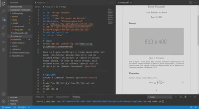
• Integrated terminal to run commands for creating documents.
• Ability to input Unicode characters. Unicode characters make writing equations easier. We can search all Unicode characters from the Unicode table. Unicode-math-symbols table contains the mappings between corresponding Unicode characters and LaTeX commands.
• Integrated PDF document viewer that refreshes the view if we create a new document. Alternatively, we can use an external PDF viewer.

For collaborative scientific writing, we recommend Authorea. Authorea is a modern web platform for scientific writing and publishing. It supports Markdown syntax, among many other modern features.

We can also write Markdown on the browser using StackEdit. It integrates with many cloud services such as Google Drive, Dropbox and GitHub. We recommend trying different editors and choosing the one that works best.

Atom

To use Atom, install it from their website and then install the following packages for writing Markdown by navigating to Edit > Preferences > Packages: language-markdown, markdown-preview-plus (disable markdown-preview), platformio-ide-terminal, pdf-view, and latex-completions.

Visual Studio Code

To use Visual Studio Code, install it from their website and then install the following extensions for writing Markdown by navigating to File > Preferences > Extensions: Markdown All in One, Markdown Preview Enhanced, and Unicode Latex. Visual Studio Code comes with an integrated terminal. Now we are ready to start creating Markdown documents.

Creating Documents

Structure

The example documents in Markdown Templates are structured as follows:

<name>/
├─ build/
├─ <filename>.md
├─ bibliography.bib
└─ Makefile

The Markdown file <filename>.md is where we write the content of the document. We use the bibliography.bib file to store bibliographical entries in BibTeX format, which we can refer to in the Markdown document.

The Makefile contains commands for converting the Markdown file into the desired document format using Pandoc. Pandoc creates the output files to the build/ directory, which Makefile automatically creates if it does not exist.

Makefile

Common

We define the build directory and the filename at the beginning of Makefile as follows.

BUILDDIR=build
FILENAME=<filename>

Then, we define the command to create the document.

<command>:
    mkdir $(BUILDDIR) -p  # Creates the BUILDDIR if it doesn't already exist.
    pandoc $(FILENAME).md \
    --filter pandoc-citeproc \
    --from=markdown+tex_math_single_backslash+tex_math_dollars \
    # ...

The option --from=markdown tells that input file is a Markdown file. Markdown extensions +tex_math_single_backslash and +tex_math_dollars enable Pandoc to parse equations.

Pandoc-citeproc enables us to use citations in Markdown. Pandoc installation includes it by default. We need to enable it by using the option --filter pandoc-citeproc.

We can execute the Makefile command in the terminal as follows.

make <command>

Next, we define concrete examples of Makefile for creating PDF, HTML, and EPUB documents.

PDF

pdf:
    mkdir $(BUILDDIR) -p  # Creates the BUILDDIR if it doesn't already exist.
    pandoc $(FILENAME).md \
    --filter pandoc-citeproc \
    --from=markdown+tex_math_single_backslash+tex_math_dollars+raw_tex \
    --to=latex \
    --output=$(BUILDDIR)/$(FILENAME).pdf \
    --pdf-engine=xelatex

Markdown extension +raw_tex enables us to insert raw LaTeX inside the Markdown document, and the --pdf-engine=xelatex option enables us to use Unicode characters within the Markdown document.

HTML

html:
    mkdir $(BUILDDIR) -p  # Creates the BUILDDIR if it doesn't already exist.
    pandoc $(FILENAME).md \
    --filter pandoc-citeproc \
    --from=markdown+tex_math_single_backslash+tex_math_dollars \
    --to=html5 \
    --output=$(BUILDDIR)/$(FILENAME).html \
    --mathjax \
    --self-contained

The --mathjax flag enables math rendering for HTML via Mathjax, and the --self-contained flag includes style sheets to the output document.

EPUB

epub:
    mkdir $(BUILDDIR) -p  # Creates the BUILDDIR if it doesn't already exist.
    pandoc $(FILENAME).md \
    --filter pandoc-citeproc \
    --from=markdown+tex_math_single_backslash+tex_math_dollars \
    --to=epub \
    --output=$(BUILDDIR)/$(FILENAME).epub \
    --epub-cover-image=<cover-image> \
    --toc

For e-books, we need to enable the table of contents needs using --toc flag. We can also include a cover image of size 1600 x 2400 pixels in JPG or PNG formats using --epub-cover-image=<cover-image> option.

Front Matter

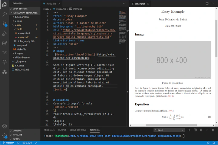
We can include document-specific metadata and functionality for the converter in the Front Matter at the top of a <filename>.md file. We write the front matter in YAML between two triple-minus lines --- as follows.

---
title: "Title"
date: \today
author: "Author"
bibliography: "bibliography.bib"
link-citations: true
urlcolor: "blue"
csl: "https://raw.githubusercontent.com/citation-style-language/styles/master/harvard-anglia-ruskin-university.csl"
---

The title, date, and author variables specify information for creating the title. The bibliography variable specifies the location of the bibliography file, link-citations toggles links to citations on and off, urlcolor defines the link color, and the csl variable defines the Citation Style Language. We can find examples of citation styles from Zotero styles and use them by either downloading them or referring directly to the URL of the raw CLS file in citation styles repository.

Layout

We can change the layout of a PDF document by including a LaTeX preamble using a Pandoc command or the Front matter. For example, if we want to create an ebook friendly PDF output, we can use the layout described in “Effort to make latex ebook friendly” as follows.

We can include --include-in-header=<layout>.tex option in the Makefile with <layout>.tex file:

\usepackage[papersize={4.5in,6in},margin=0.5cm]{geometry}
\setlength{\parskip}{2pt}
\newcommand\textbreak{%
  \begin{center}%
  \decothreeleft \aldineleft \decosix \aldineright \decothreeright%
  \end{center}}
\pagestyle{empty}

Alternatively, we can include the header-includes variable in the front matter:

header-includes: |
    \usepackage[papersize={4.5in,6in},margin=0.5cm]{geometry}
    \setlength{\parskip}{2pt}
    \newcommand\textbreak{%
    \begin{center}%
    \decothreeleft \aldineleft \decosix \aldineright \decothreeright%
    \end{center}}
    \pagestyle{empty}    

Syntax

Basic Syntax

John Gruber’s original spec and Markdown Cheatsheet in GitHub demonstrate the basic Markdown syntax. We recommend reading at least them to understand the basics. In addition to Markdown understanding, basics on HTML can be useful for creating web content if using inline HTML.

Code Blocks

Regular Markdown supports code blocks but does not highlight their syntax. However, converters such as Pandoc will add syntax highlighting for code block as long as we supply the appropriate language for the code block. For example:

```python
def foo():
    return "bar"
```

Displays as:

def foo():
    return "bar"

Equations

We can write inline equations using single dollars $...$ or backslashed parentheses \(...\) and display using double dollars $$...$$ or backslashed square brackets \[...\]. The use of dollar symbols is more common. Optionally, we can add tags \tag{<tag>} for numbering equations and labels \label{<label>} for referring to equations later in text using \ref{<label>}. For example, we can write Cauchy’s integral formula as

$$
f(a)={\frac {1}{2\pi i}}\oint _{\gamma }{\frac {f(z)}{z-a}}\,dz
\tag{1}
\label{1}
$$

Mathjax displays the equation as

We can now refer to the equation using syntax (\ref{1}) which displays as (\ref{1}). Markdown displays inline equations such as $a^2+b^2=c^2$ in the same line as the text, $a^2 + b^2 = c^2.$

Some markdown parsers do not detect the equation mode for characters that are part of the Markdown syntax, which might interfere with parsing. For example, instead of using the asterisk symbol * inside the equation mode, we can use the backslashed ASCII \*, latex command \ast, or the Unicode version ∗.

Unicode Symbols for Equations

We write equations easier by using Unicode characters for mathematical symbols. For example, instead of \mathbf{x}\in\mathbb{R}^2 we can write $𝐱∈ℝ^2$ for the same output $𝐱∈ℝ^2$. You can input Unicode symbols with editor plugins mentioned in the Editors section.

Colored Equations

Better Explained in their article Colorized Math Equations shows how to use colors to improve the way we can describe equations. The article has excellent examples, such as a colorized explanation for the constant $e,$ which they also provide as a LaTeX document. We can use it to recreate the output on the web:

$\growth \text{The base for continuous growth}$ $\plain \text{is}$ $\unitQuantity \text{the unit quantity}$ $\unitInterest \text{earning unit interest}$ $\unitTime \text{for unit time,}$ $\compounded \text{compounded}$ $\perfectly \text{as fast as possible}.$

To use colors in LaTeX, we must include the color package in the header.

\usepackage{color}

Then, we can define new colors in the body and use them in math mode. For example:

\definecolor{c1}{RGB}{114,0,172}
\newcommand{\newcolor}{\color{c1}}
$$
\newcolor x^2
$$

Overleaf has a helpful article about Using colors in LaTeX.

When using Mathjax or KaTeX to render equations on the web, we can use the extended color keywords or RBG hex values for the color argument. The commands must be inside math mode.

We can define colors using the \color command.

$$
\newcommand{\positive}{\color{darkblue}}
\newcommand{\negative}{\color{darkred}}
{\positive α} {\negative -β}, \quad ∀α,β>0
$$

Alternatively, we can define the colors using the \textcolor command.

$$
\newcommand{\positive}[1]{\textcolor{darkblue}{#1}}
\newcommand{\negative}[1]{\textcolor{darkred}{#1}}
\positive{α} \negative{-β}, \quad ∀α,β>0
$$

We can take into account color blindness by using a colorblind safe palette. We can use Colorbrewer, a tool for coloring planar graphs (aka maps), to select different colorblind safe palettes. In Colorbrewer, choose the colorblind safe option, select the color scheme from sequential or diverging, the number of data classes and HEX or RGB output. Finally, copy the color codes from the bottom left to the LaTeX commands.

Citations

Let us have the following BibTeX entry stored in bibliography.bib file.

@article{key_name,
    author  = {Peter Adams},
    title   = {The title of the work},
    journal = {The name of the journal},
    year    = {1993},
    number  = {2},
    pages   = {201-213},
    month   = {7},
    note    = {An optional note},
    volume  = {4}
}

We can refer to this entry in the Markdown document using syntax @key_name or [@key_name]. Pandoc creates references at the bottom of the document.

Vector Graphics

Markdown allows inserting vector graphics with the standard syntax.

![](<filename>.svg)

Using vector graphics when creating PDFs requires Inkscape.

Conclusion

I wrote this article based on my experiences of writing scientific essays and handouts, technical documentation, and blog articles. I hope it helps you to write these types of documents more effectively.

If need resources for faster, more comfortable typing, I recommend the Keyboard section on the Ergonomic Workstation page. For improving your grammar and editing text, you can check out my Digital Writing page.

Contribute

If you enjoyed or found benefit from this article, it would help me share it with other people who might be interested. If you have feedback, questions, or ideas related to the article, you can contact me via email. For more content, you can follow me on YouTube or join my newsletter. Creating content takes time and effort, so consider supporting me with a one-time donation.