Noise Filtering Using 1€ Filter
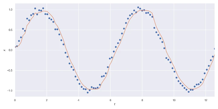
Table of Contents
Introduction
This article explores the 1€ Filter, a simple, but powerful algorithm for filtering noisy real-time signals. The article focuses on the practical implementation of the algorithm, and it covers the mathematical basis, a pseudocode implementation, and simple, pure Python implementation of the algorithm. To understand why and how the filter works, we recommend reading the original article 1.
1€ Filter
The 1€ Filter is a low pass filter for filtering noisy signals in real-time. It is also a simple filter with only two configurable parameters. The signal at time $T_i$ is denoted as value $X_i$ and the filtered signal as value $\hat{X}_i$. The filter uses exponential smoothing
$$\hat{X}_1 = X_1$$ $$\hat{X}_i = α X_i + (1-α) \hat{X} _{i-1},\quad i≥2 \tag{1} \label{1} $$where the smoothing factor $α∈[0, 1]$, instead of being a constant, is adaptive, that is, dynamically computed using information about the rate of change (speed) of the signal. The adaptive smoothing factor aims to balance the jitter versus lag trade-off since people are sensitive to jitter at low speeds and more sensitive to lag at high speeds. The smoothing factor is defined as
$$α = \frac{1}{1 + \dfrac{τ}{T_e}},$$where $T_e$ is the sampling period computed from the time difference between the samples
$$T_e=T_i-T _{i-1}$$and $τ$ is time constant computed using the cutoff frequency
$$τ = \frac{1}{2πf_C}.$$The cutoff frequency $f_C$ increases linearly as the rate of change, aka speed, increases
$$f_C=f_{C_{min}} + β|\hat{\dot{X}}_i|$$where $f _{C _{min}}>0$ is the minimum cutoff frequency, $β>0$ is the speed coefficient and $\hat{\dot{X}}_i$ is the filtered rate of change. We define the rate of change $\hat{X}_i$ as the discrete derivative of the signal
$$\dot{X}_1 = 0$$ $$\dot{X}_i = \frac{X_i-\hat{X} _{i-1}}{T_e},\quad i≥2$$which is then filtered using exponential smoothing $\eqref{1}$ with a constant cutoff frequency $f_{C_d},$ by default $f_{C_d}=1$.
Algorithm
In this section, we implement the 1€ filter algorithm as pseudocode. The precise implementation of the algorithm depends on the programming language and paradigm in question. We have written this algorithm using a functional style.
$\operatorname{Smoothing-Factor}(f_C, T_e)$- $r=2π⋅f_c⋅T_e$
- return $\dfrac{r}{r+1}$
- return $α X_i + (1-α) \hat{X}_{i-1}$
- $T_e=T_i-T_{i-1}$
- $α_d=\operatorname{Smoothing-Factor}(T_e, f_{C_d})$
- $\dot{X}_i = \dfrac{X_i-\hat{X} _{i-1}}{T_e}$
- $\hat{\dot{X}}_i=\operatorname{Exponential-Smoothing}(α_d, \dot{X}_i, \hat{\dot{X}} _{i-1})$
- $f_C=f_{C_{min}} + β|\hat{\dot{X}}_i|$
- $α=\operatorname{Smoothing-Factor}(f_C, T_e)$
- $\hat{X}_i=\operatorname{Exponential-Smoothing}(α, X_i, \hat{X} _{i-1})$
- return $T_i,\hat{X}_i,\hat{\dot{X}}_i$
Tuning the Filter
There are two configurable parameters in the model, the minimum cutoff frequency $f _{C _{min}}$ and the speed coefficient $β$. Decreasing the minimum cutoff frequency decreases slow speed jitter. Increasing the speed coefficient decreases speed lag.
Python Implementation
The following Python implementation is available in the OneEuroFilter GitHub repository.
The object-oriented approach stores the previous values inside the object instead of explicitly giving them a return value as functional implementation would. It should be relatively simple to implement this algorithm in other languages.
import math


def smoothing_factor(t_e, cutoff):
    r = 2 * math.pi * cutoff * t_e
    return r / (r + 1)


def exponential_smoothing(a, x, x_prev):
    return a * x + (1 - a) * x_prev


class OneEuroFilter:
    def __init__(self, t0, x0, dx0=0.0, min_cutoff=1.0, beta=0.0,
                 d_cutoff=1.0):
        """Initialize the one euro filter."""
        # The parameters.
        self.min_cutoff = float(min_cutoff)
        self.beta = float(beta)
        self.d_cutoff = float(d_cutoff)
        # Previous values.
        self.x_prev = float(x0)
        self.dx_prev = float(dx0)
        self.t_prev = float(t0)

    def __call__(self, t, x):
        """Compute the filtered signal."""
        t_e = t - self.t_prev

        # The filtered derivative of the signal.
        a_d = smoothing_factor(t_e, self.d_cutoff)
        dx = (x - self.x_prev) / t_e
        dx_hat = exponential_smoothing(a_d, dx, self.dx_prev)

        # The filtered signal.
        cutoff = self.min_cutoff + self.beta * abs(dx_hat)
        a = smoothing_factor(t_e, cutoff)
        x_hat = exponential_smoothing(a, x, self.x_prev)

        # Memorize the previous values.
        self.x_prev = x_hat
        self.dx_prev = dx_hat
        self.t_prev = t

        return x_hat
Code for the plot:
import matplotlib.pyplot as plt
import numpy as np
import seaborn
from matplotlib.animation import FuncAnimation

from one_euro_filter import OneEuroFilter


np.random.seed(1)

# Parameters
frames = 100
start = 0
end = 4 * np.pi
scale = 0.05


# The noisy signal
t = np.linspace(start, end, frames)
x = np.sin(t)
x_noisy = x + np.random.normal(scale=scale, size=len(t))


# The filtered signal
min_cutoff = 0.004
beta = 0.7
x_hat = np.zeros_like(x_noisy)
x_hat[0] = x_noisy[0]
one_euro_filter = OneEuroFilter(
    t[0], x_noisy[0],
    min_cutoff=min_cutoff,
    beta=beta
)
for i in range(1, len(t)):
    x_hat[i] = one_euro_filter(t[i], x_noisy[i])


# The figure
# https://eli.thegreenplace.net/2016/drawing-animated-gifs-with-matplotlib/
seaborn.set()
fig, ax = plt.subplots(figsize=(12, 6))
ax.set(
    xlim=(start, end),
    ylim=(1.1*(-1-scale), 1.1*(1+scale)),
    xlabel="$t$",
    ylabel="$x$",
)
fig.set_tight_layout(True)
signal, = ax.plot(t[0], x_noisy[0], 'o')
filtered, = ax.plot(t[0], x_hat[0], '-')


def update(i):
    print(i)
    signal.set_data(t[0:i], x_noisy[0:i])
    filtered.set_data(t[0:i], x_hat[0:i])
    return signal, filtered


if __name__ == '__main__':
    # FuncAnimation will call the 'update' function for each frame; here
    # animating over 10 frames, with an interval of 200ms between frames.
    anim = FuncAnimation(fig, update, frames=frames, interval=100)
    anim.save('one_euro_filter.gif', dpi=80, writer='imagemagick')
    # update(frames)
    plt.savefig("one_euro_filter.png", dpi=300)
Conclusions
I first learned about the 1€ filter at Computational User Interface Design course at Aalto University. I found the algorithm to be elegant, but the original paper’s explanation was cumbersome for implementing it. It motivated me to create a simplified explanation and code to help other people implement this algorithm.
Contribute
If you enjoyed or found benefit from this article, it would help me share it with other people who might be interested. If you have feedback, questions, or ideas related to the article, you can contact me via email. For more content, you can follow me on YouTube or join my newsletter. Creating content takes time and effort, so consider supporting me with a one-time donation.
References
Casiez, G., Roussel, N., & Vogel, D. (2012). 1€ filter: a simple speed-based low-pass filter for noisy input in interactive systems. In Proceedings of the SIGCHI Conference on Human Factors in Computing Systems (pp. 2527–2530). ↩︎
Jaan Tollander de Balsch
Jaan Tollander de Balsch is a computational scientist with a background in computer science and applied mathematics.