Exploring the Pointwise Convergence of Legendre Series for Piecewise Analytic Functions
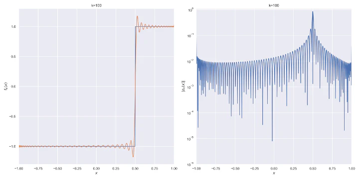
Table of Contents
Introduction
In this article, we explore the behavior of the pointwise convergence of the Legendre series for piecewise analytic functions using numerical methods. The article extensively covers the mathematics required for forming and computing the series as well as pseudocode code for some of the non-trivial algorithms. It extends the research made in the papers by Babuska and Hakula 1 2 by proving evidence for the conjectures about the Legendre series in a large number of points in the domain and up to very high degree series approximations. We present the numerical results as figures and provide explanations. We also provide the Python code for computing and recreating the results in LegendreSeries repository.
Legendre Polynomials
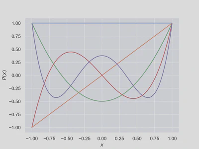
Legendre polynomials are a system of complete and orthogonal polynomials defined over the domain $Ω=[-1, 1]$ which is an interval between the edges $-1$ and $1$, as a recursive formula
$$P_{0}(x) = 1$$
$$P_{1}(x) = x$$
$$P_{n}(x) = \frac{2n-1}{n} x P_{n-1}(x) - \frac{n-1}{n} P_{n-2}(x), n≥2. \tag{1} \label{recursive-formula}$$
The recursive definition enables efficient computing of numerical values of high degree Legendre polynomials at specific points in the domain.
Legendre polynomials also have important properties which are used for forming the Legendre series. The terminal values, i.e. the values at the edges, of Legendre polynomials can be derived from the recursive formula
$$P_{n}(1) = 1$$
$$P_{n}(-1) = (-1)^n. \tag{2} \label{terminal-values} $$
The symmetry property also follows from the recursive formula
$$P_n(-x) = (-1)^n P_n(x). \tag{3} \label{symmetry}$$
The inner product is denoted by the angles
$$⟨P_m(x), P_n(x)⟩ _{2} = \int _{-1}^{1} P _m(x) P _n(x) dx$$
$$= \frac{2}{2n + 1} δ _{mn}, \tag{4} \label{inner-product} $$
where $δ_{mn}$ is Kronecker delta.
Differentiation of Legendre polynomials can be defined in terms of Legendre polynomials themselves as
$$ (2n+1) P_n(x) = \frac{d}{dx} \left[ P_{n+1}(x) - P_{n-1}(x) \right]. \tag{5} \label{differentiation-rule} $$
The differentiation $\eqref{differentiation-rule}$ rule can also be formed into the integration rule
$$ ∫P_n(x)dx = \frac{1}{2n+1} (P_{n+1}(x) - P_{n-1}(x)). \tag{6} \label{integration-rule} $$
Legendre Series
The Legendre series is a series expansion which is formed using Legendre polynomials. Legendre series of function $f$ is defined as
$$ f(x) = ∑{n=0}^{∞}C{n}P_{n}(x). \tag{7} \label{legendre-series} $$
where $C_n∈ℝ$ are the Legendre series coefficients and $P_n(x)$ Legendre polynomials of degree $n$. The formula for the coefficients is defined
$$ C_n = \frac{2n+1}{2} \int_{-1}^{1} f(x) P_{n}(x)dx. \tag{8} \label{legendre-series-coefficients} $$
The Legendre series coefficients can be derived using the Legendre series formula $\eqref{legendre-series}$ and the inner product $\eqref{inner-product}$.
Show proof:
$$f(x) = ∑{m=0}^{∞}C{m}P_{m}(x)$$ $$P_{n}(x) f(x) = P_{n}(x) \sum {m=0}^{\infty }C{m}P_{m}(x)$$ $$∫{-1}^{1}P{n}(x) f(x)dx = ∫{-1}^{1} P{n}(x) \sum {m=0}^{\infty }C{m}P_{m}(x)dx$$ $$∫{-1}^{1}P{n}(x) f(x)dx = \sum {m=0}^{\infty }C{m}∫{-1}^{1} P{n}(x) P_{m}(x)dx$$ $$∫{-1}^{1}P{n}(x) f(x)dx = C_{n}∫{-1}^{1} P{n}(x) P_{n}(x)dx$$ $$C_{n} = {\langle f,P {n}\rangle {2} \over |P {n}|{2}^{2}}$$ $$C_n = \frac{2n+1}{2} \int{-1}^{1} f(x) P{n}(x)dx.$$
The partial sum of the series expansion gives us an approximation of the function $f$. It’s obtained by limiting the series to a finite number of terms $k$
$$ f_k(x)=\sum _{n=0}^{k}C _{n}P _{n}(x). \tag{9} \label{partial-sum} $$
The approximation error $ε_k$ is obtained by subtracting the partial sum $f_k$ from the real value of the function $f$
$$ ε_k(x) = f(x)-f_k(x). \tag{10} \label{approximation-error} $$
The actual analysis of the approximation errors will be using the absolute value of the error $|ε_k(x)|.$
Piecewise Analytic Functions
The motivation for studying a series expansion for piecewise analytic functions is to understand the behavior of a continuous approximation of a function with non-continuous or non-differentiable points. We will study the series expansion on two special cases of piecewise analytic functions, the step function and the V function. The results obtained from studying these two special cases generalizes into all piecewise analytic functions, but this is not proven here.
Piecewise analytic function $f(x):Ω → ℝ$ is defined
$$ f(x) = \sum_{i=1}^{m} c_i | x-a_i |^{b_i} + v(x), \tag{11} \label{piecewise-analytic-function} $$
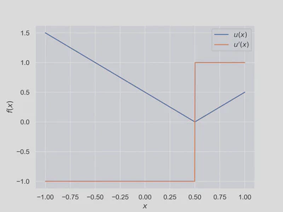
where $a_i∈(-1,1)$ are the singularities, $b_i∈ℕ_0$ are the degrees, $c_i∈ℝ$ are the scaling coefficients and $v(x)$ is an analytic function. The V function is piecewise analytic function of degree $b=1$ and it is defined as
$$ u(x) = c ⋅ |x - a| + (α + βx). \tag{12} \label{v-function} $$
The step function is piecewise analytic function of degree $b=0$ and it is obtained as the derivative of the V-function
$$ \frac{d}{dx} u(x) = u’(x) = c ⋅ \operatorname{sign}{(x - a)} + β. \tag{13} \label{step-function} $$
As can be seen, the V function is the absolute value scaled with $c$, translated with $α$ and rotated by $βx$ and the step function is sign function that is scaled with $c$ and translated with $β$.
We’ll also note that the derivative of step function is zero
$$ \frac{d}{dx} u’(x) = u’’(x) = 0. \tag{14} \label{step-function-derivative} $$
This will be used when forming the Legendre series.
Legendre Series of Step Function
The coefficients for the Legendre series of the step function will be referred as step function coefficients. A formula for them in terms of Legendre polynomials at the singularity $a$ can be obtained by substituting the step function $\eqref{step-function}$ in place of the function $f$ in the Legendre series coefficient formula $\eqref{legendre-series-coefficients}$
$$A_n = \frac{2n+1}{2} \int_{-1}^{1} u’(x) P_{n}(x)dx \tag{15} \label{step-function-coefficients} $$
$$A_0 = β-ac$$
$$A_n = c(P_{n-1}(a)-P_{n+1}(a)),\quad n≥1$$
Proof: The coefficients for degree $n=0$ are obtained from direct integration
$$A_{0} = \frac{1}{2} \int_{-1}^{1} u^{\prime}(x) dx$$ $$= \beta + \frac{1}{2} c \int_{-1}^{1} \operatorname{sign}{\left (x - a \right )}dx$$ $$= \beta + \frac{1}{2} c \left(\int_{-1}^{a} -1dx + \int_{a}^{1} 1dx\right)$$ $$= \beta - ac. \tag{16} \label{step-function-coefficients-0} $$
The coefficients for degrees $n≥1$ are obtained by using integration by parts, integral rule $\eqref{integration-rule}$, terminal values $\eqref{terminal-values}$ and the derivative of step function $\eqref{step-function-derivative}$
$$A_{n} = \frac{2n+1}{2} \int_{-1}^{1} u^{\prime}(x) P_{n}(x)dx, n≥1$$
$$= \frac{2n+1}{2} \left( \left[u^\prime(x) \int P _n(x) dx\right] _{-1}^{1} - \int _{-1}^{1} u^{\prime\prime}(x) P _n(x) dx \right)$$
$$= \frac{2n+1}{2} \left[ \frac{1}{2n+1} (P_{n+1}(x) - P_{n-1}(x)) u^\prime(x) \right]_{-1}^{1}$$
$$= \frac{1}{2} \left[ (P_{n+1}(x) - P_{n-1}(x)) u^\prime(x) \right]_{-1}^{1}$$
$$\begin{aligned}= & \frac{1}{2} \left[ (P_{n+1}(x) - P_{n-1}(x)) u^\prime(x) \right]{-1}^{a} + \\ & \frac{1}{2} \left[ (P{n+1}(x) - P_{n-1}(x)) u^\prime(x) \right]_{a}^{1} \end{aligned}$$
$$\begin{aligned}= & \frac{1}{2} \left[ (P_{n+1}(x) - P_{n-1}(x)) \cdot (-c+\beta) \right]{-1}^{a} + \\ & \frac{1}{2} \left[ (P{n+1}(x) - P_{n-1}(x)) \cdot (c+\beta) \right]_{a}^{1} \end{aligned}$$
$$= c \cdot \left(P_{n-1}(a) - P_{n+1}(a)\right). \tag{17} \label{step-function-coefficients-n} $$
Legendre Series of V Function
The coefficients for the Legendre series of the step function will be referred as V function coefficients. A formula for them in terms of step function coefficients can be obtained by substituting the V function $\eqref{v-function}$ in place of the function $f$ in the Legendre series coefficient formula $\eqref{legendre-series-coefficients}$
$$B_n = \frac{2n+1}{2} \int_{-1}^{1} u(x) P_{n}(x)dx. \tag{18} \label{v-function-coefficients} $$
$$B_0 = \frac{a^{2} c}{2} + α + \frac{c}{2}$$
$$B_n=-\frac{A_{n+1}}{2n +3} + \frac{A_{n-1}}{2n - 1},\quad n≥1$$
Proof: The coefficients for degree $n=0$ are obtained from direct integration
$$ B_{0} = \frac{1}{2} ∫_{-1}^{1} u(x) dx = \frac{a^{2} c}{2} + α + \frac{c}{2}. \tag{19} \label{v-function-coefficients-0} $$
The coefficients for degrees $n≥1$ are obtained by using integration by parts, integral rule $\eqref{integration-rule}$ and substituting the step function coefficient formula $\eqref{step-function-coefficients}$
$$B_{n} = \frac{2n+1}{2} \int_{-1}^{1} u(x) P_{n}(x) dx, \quad n \geq 1 $$ $$= \frac{2n + 1}{2} \left ( \left [ u(x) \int P_n(x) dx \right ]{-1}^{1} - \int{-1}^{1} u’(x) \int P_{n} dx dx \right ) $$ $$= -\frac{1}{2} \int_{-1}^{1} \left [ P_{n+1}(x) - P_{n-1}(x) \right ] u’(x) dx$$ $$= -\frac{1}{2} \int_{-1}^{1} P_{n+1}(x) u’(x) dx + \frac{1}{2} \int_{-1}^{1} P_{n-1}(x) u’(x) dx.$$ $$= -\frac{A_{n+1}}{2n +3} + \frac{A_{n-1}}{2n - 1}. \tag{20} \label{v-function-coefficients-n} $$
Pointwise Convergence

The series is said to converge pointwise if the partial sum $f_k(x)$ tends to the value $f(x)$ as the degree $k$ approaches infinity in every $x$ in the domain $Ω$
$$ \lim_{k→∞} f_k(x)=f(x). \tag{21} \label{pointwise_convergence} $$
Equivalently in terms of the approximation error which approaches zero
$$ \lim_{k→∞} ε_k(x)=0. \tag{22} \label{approximation_error_convergence} $$
Numerical exploration of the pointwise convergence explores the behavior of the approximation error $ε_k(x)$ as a function of degree $k$ up to a finite degree $n$ at some finite amount of points $x$ selected from the domain $Ω.$ The numerical approach answers to how the series converges contrary to the analytical approach which answers if the series converges.
Convergence Line
We will perform the exploration by computing a convergence line which contains two parameters:
The convergence rate which is the maximal rate at which the error approaches zero as the degree grows.
The convergence distance which is a value proportional to the degree when the series reaches the maximal rate of convergence.
The definition of the converge line requires a definition for a line. A line between two points $(x_0,y_0)$ and $(x_1,y_1)$ where $x_0≠x_1$ is defined as
$$ y=(x-x_{0}),{\frac {y_{1}-y_{0}}{x_{1}-x_{0}}}+y_{0}. \tag{23} \label{line1} $$
An alternative form of this formula is
$$ y=\tilde{a}x+\tilde{β}, \tag{24} \label{line2} $$
where the coefficient $\tilde{α}=\frac{y _{1}-y _{0}}{x _{1}-x _{0}}$ is referred as the slope and the coefficient $\tilde{β}=(y _{0}-x _{0}\tilde{α})$ is referred as the intercept.
The pseudocode for the convergence line algorithm is then as follows:
Input: A sequence of strictly monotonically increasing positive real numbers $(x_1,x_2,…,x_n)$ and a sequence of positive real numbers $(y_1,y_2,…,y_n)$ that converges towards zero (decreasing). Limit for the smallest value of the slope $\tilde{α}_{min}$.
Output: A convergence line defined by the values $\tilde{α}$ and $\tilde{β}$ which minimizes $\tilde{α}$ and minimizes $\tilde{β}$ such that $\tilde{α}≥\tilde{α}_{min}$ and $y_i=\tilde{α}x_i+\tilde{β}$ for all $i=1,2,…,n.$
$\operatorname{Find-Convergence-Line}((x_1,x_2,…,x_n),(y_1,y_2,…,y_n),\tilde{α}_{min})$
- $i=1$
- $j=i$
- while $j≠n$
- ….. $k=\underset{k>j}{\operatorname{argmax}}\left(\dfrac{y_k-y_j}{x_k-x_j}\right)$
- ….. $\tilde{α} = \dfrac{y_k-y_j}{x_k-x_j}$
- ….. if $\tilde{α} < \tilde{α}_{min}$
- ….. ….. break
- ….. $i=j$
- ….. $j=k$
- $\tilde{α}=\dfrac{y_j-y_i}{x_j-x_i}$
- $\tilde{β}=y_i-x_i \tilde{α}$
- return $(\tilde{α}, \tilde{β})$
The approximation errors generated by the Legendre series have linear convergence in the logarithmic scale, and therefore we need to convert the values into a logarithmic scale, find the convergence line and then convert the line into exponential form $βx^{-α}$.
Input: The degrees $(k_1,k_2,…,k_n)$ corresponding to the approximation errors $(ε_1,ε_2,…,ε_n)$ generated by a series and the limit $\tilde{α}_{min}$.
Output: The coefficient $α$ correspond to the rate of convergence, and the coefficient $β$ corresponds to the distance of convergence such that $ε_k≤βk_i^{-α}$ for all $i=1,2,…,n.$
$\operatorname{Find-Convergence-Line-Log}((k_1,k_2,…,k_n),(ε_1,ε_2,…,ε_n),a_{min})$
- $x=(\log_{10}(k_1),\log_{10}(k_2),…,\log_{10}(k_n))$
- $y=(\log_{10}(|ε_1|,\log_{10}(|ε_2|,…,\log_{10}(|ε_n|))$
- $(\tilde{α},\tilde{b})=\operatorname{Find-Convergence-Line}(x,y,\tilde{α}_{min})$
- $α=-\tilde{α}$
- $β=10^\tilde{β}$
- return $(α,β)$
Conjectures of Pointwise Convergence
The papers by Babuska and Hakula 1 2 introduced two conjectures about the convergence rate and convegence distance. They are stated as follows. The convergence rate $α$ depends on $x$ and the degree $b$
$$ α(x,b)= \begin{cases} \max(b,1), & x=a \\ b+1/2, & x∈\{-1,1\} \\ b+1, & x∈(-1,a)∪(a,1). \\ \end{cases} \tag{25} \label{convergence-rate} $$
As can be seen, there are different convergence rates at the edges, singularity and elsewhere.
The convergence distance $β$ depends on $x$ but is independent of the degree $b.$ Near singularity we have
$$ β(a±ξ)≤Dξ^{-ρ}, ρ=1 \tag{26} \label{convergence-distance-near-singularity} $$
and near edges we have
$$ β(±(1-ξ))≤Dξ^{-ρ}, ρ=1/4 \tag{27} \label{convergence-distance-near-edges} $$
where $ξ$ is small positive number and $D$ is a positive constant. The behaviour near the singularity is related to the Gibbs phenomenom.
Results
The source code for the algorithms, plots, and animations is available in the LegendreSeries GitHub repository. It also contains instructions on how to run the code.
The results were obtained by computing the approximation error $\eqref{approximation-error}$ for the step function and V function up to degree $n=10^5.$ The values of $x$ from the domain $Ω$ were chosen to include the edges, singularity, and its negation, zero, points near the edges and singularity, and points elsewhere in the domain. Then pointwise convergence was analyzed by finding the convergence line, i.e., the values for the rate of convergence $α$ and the distance of convergence $β$ for the approximation errors. The values were then verified to follow the conjectures $\eqref{convergence-rate}$, $\eqref{convergence-distance-near-edges}$ and $\eqref{convergence-distance-near-singularity}$ as can be seen from the figures below.
Step Function
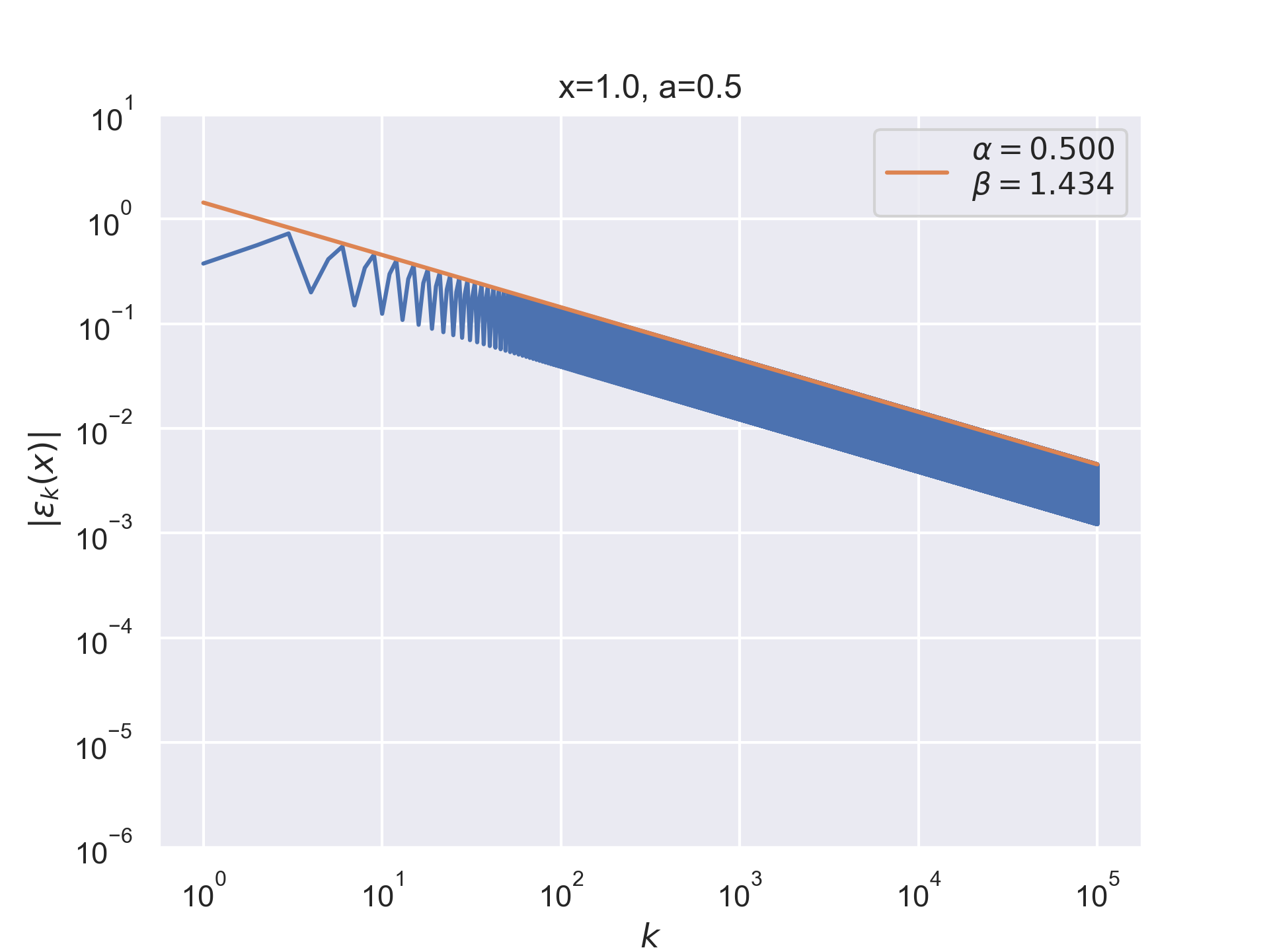
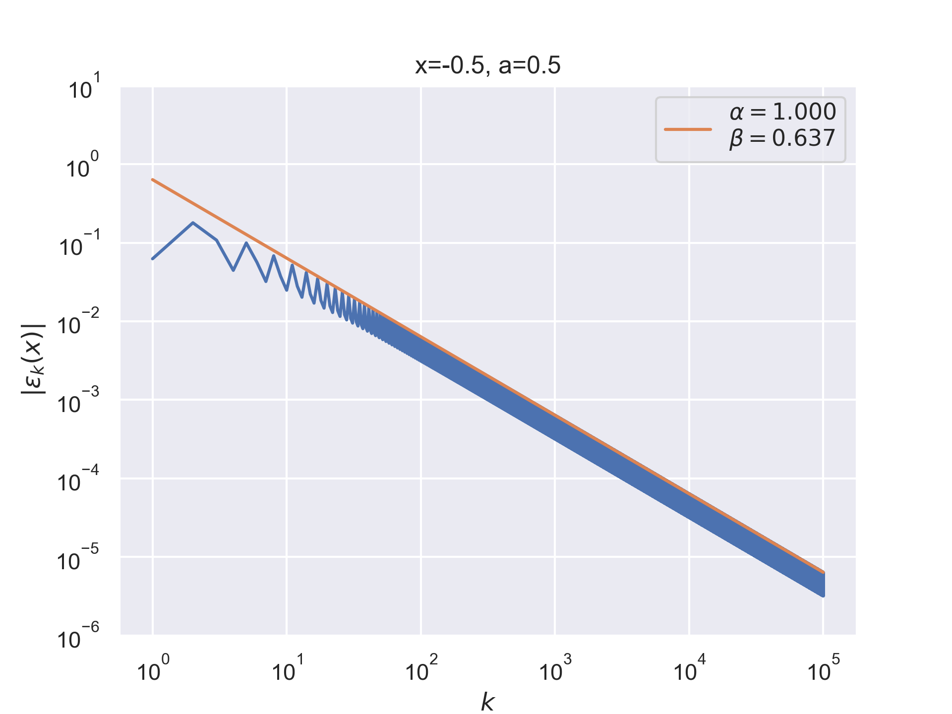
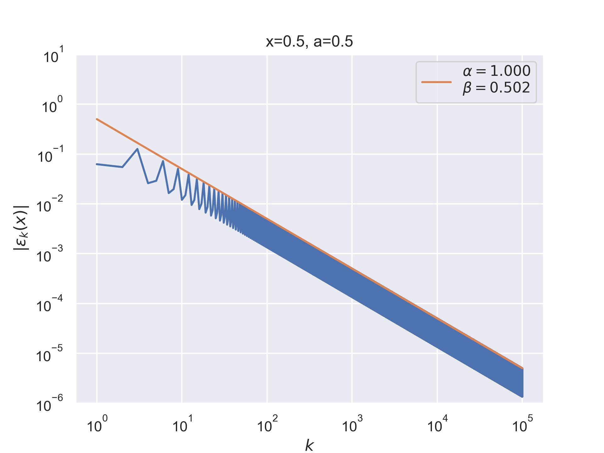
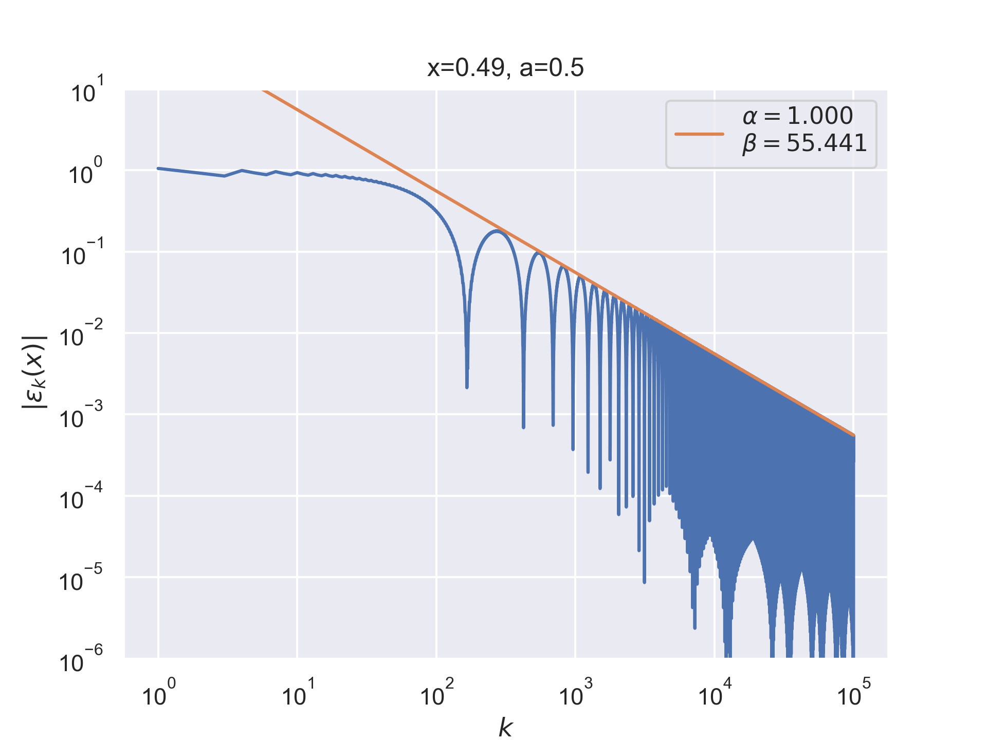
The following results where $a=0.5$ and $b=0$ for the step function.
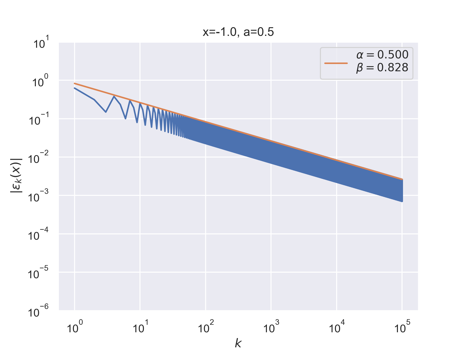
Pointwise convergence at the edges has a convergence rate of $α=1/2$.
Pointwise convergence at the singularity and its negation have a convergence rate of $α=1$.
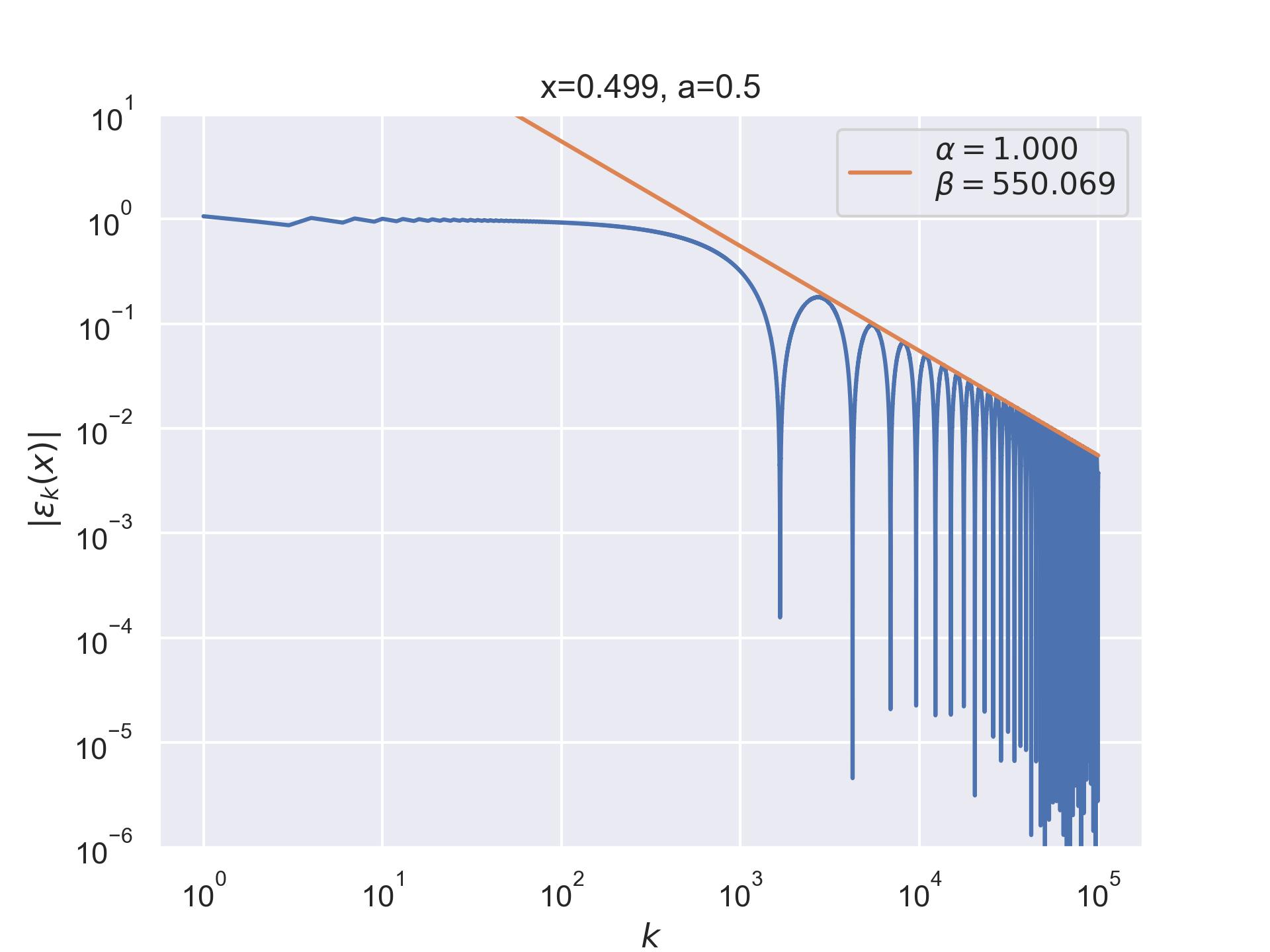
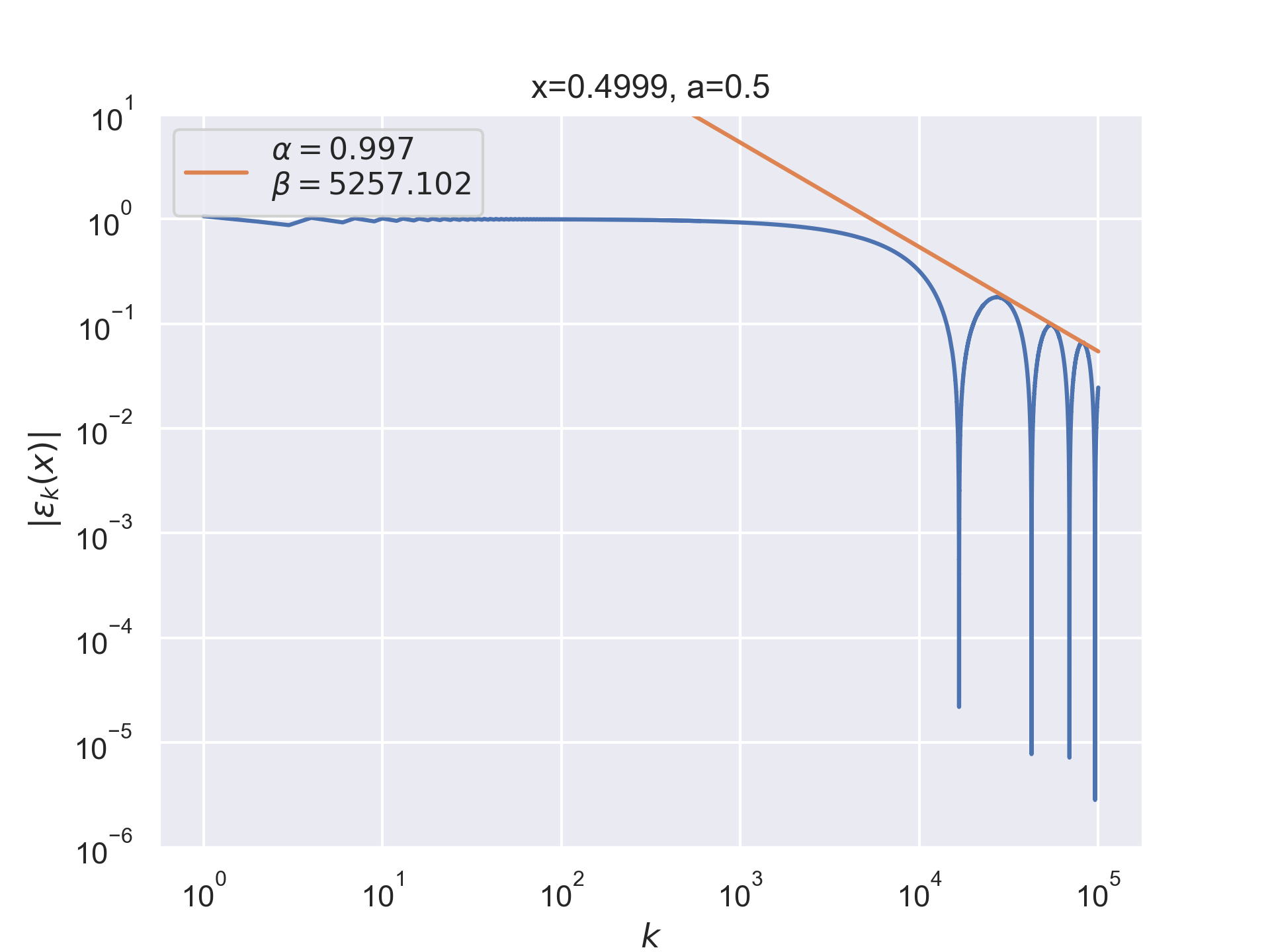
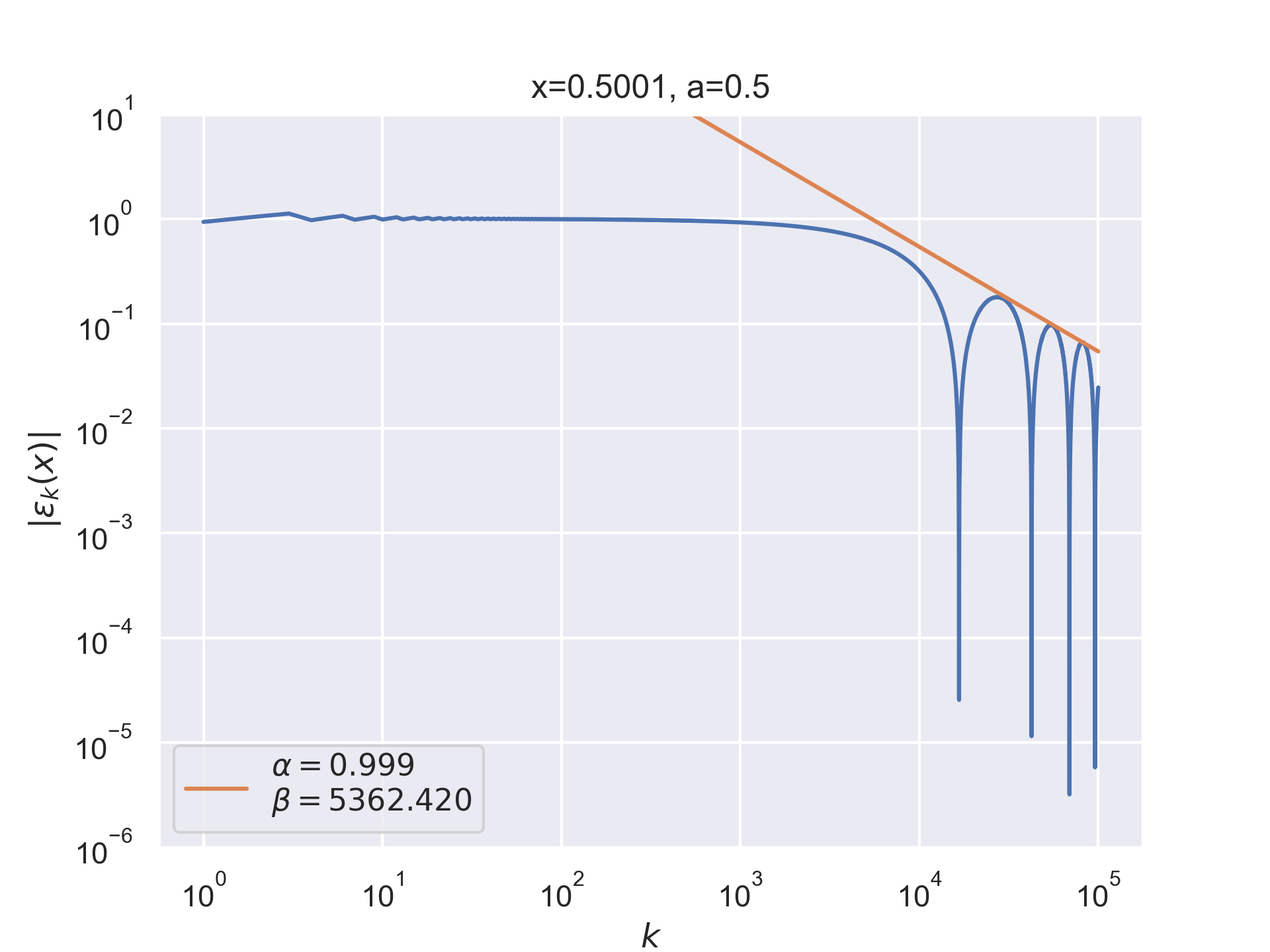

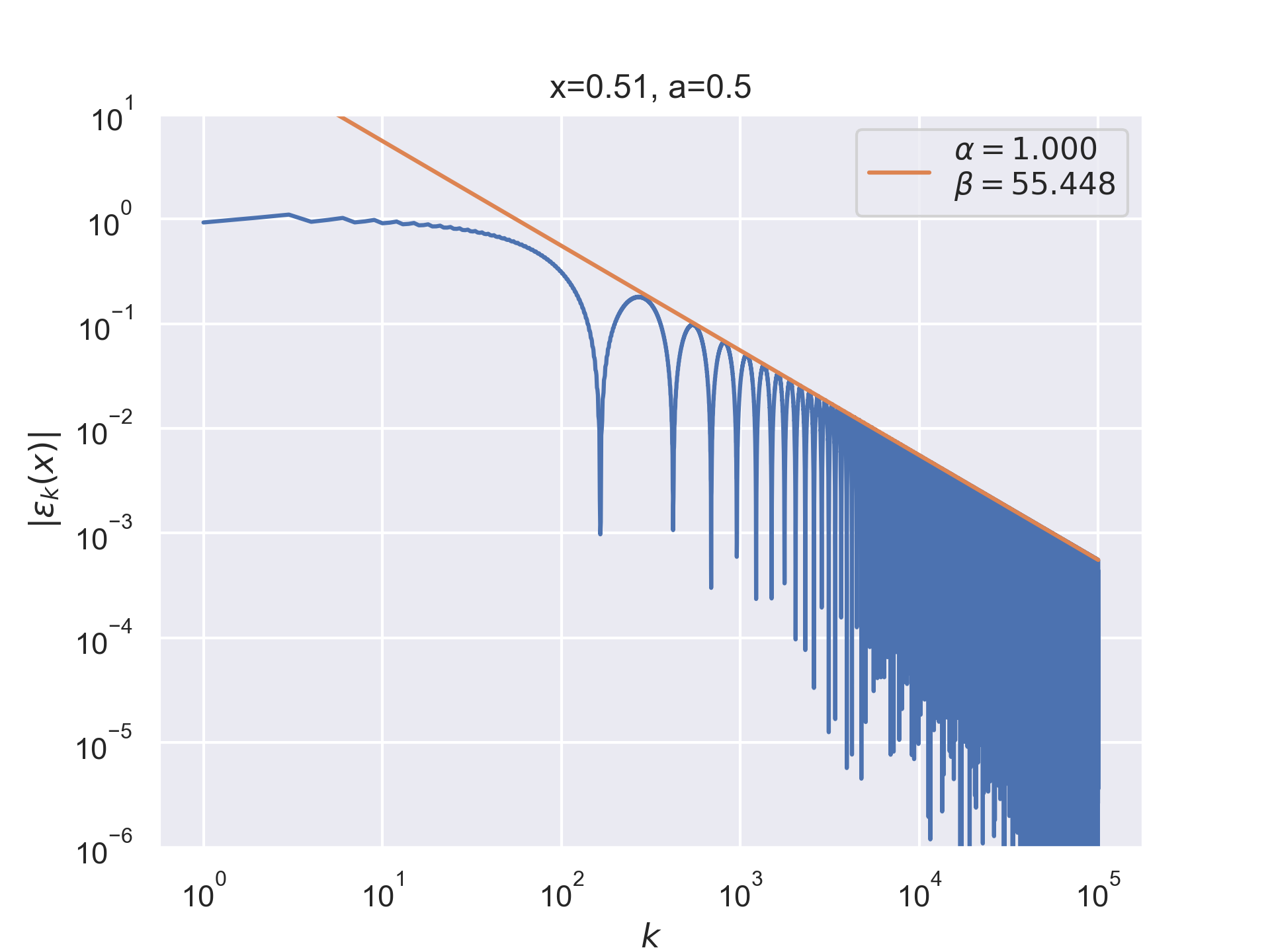
Pointwise convergence near singularity $a±ξ$ has a rate of convergence $α=1$, but as can be seen, the distance of convergence $β$ increases as $x$ moves closer to the singularity from either side.
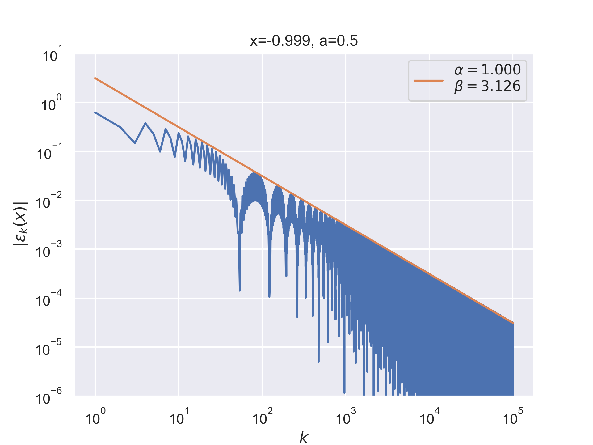
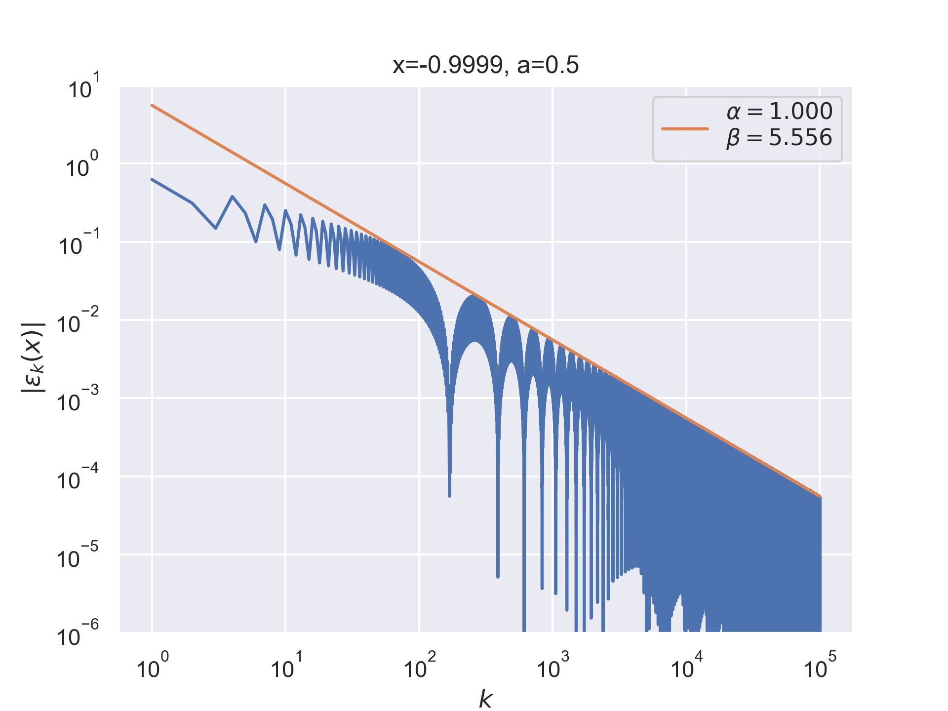
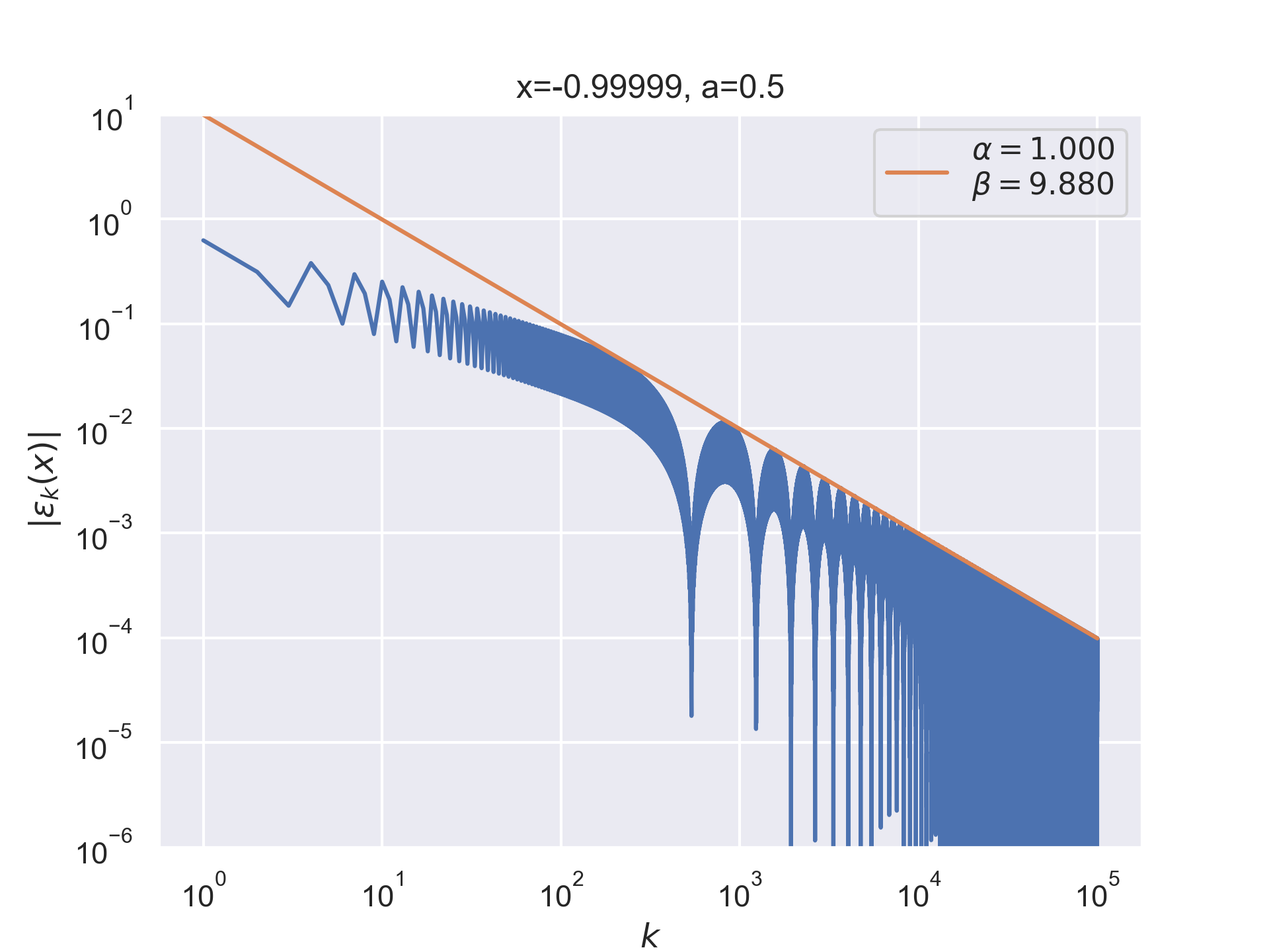
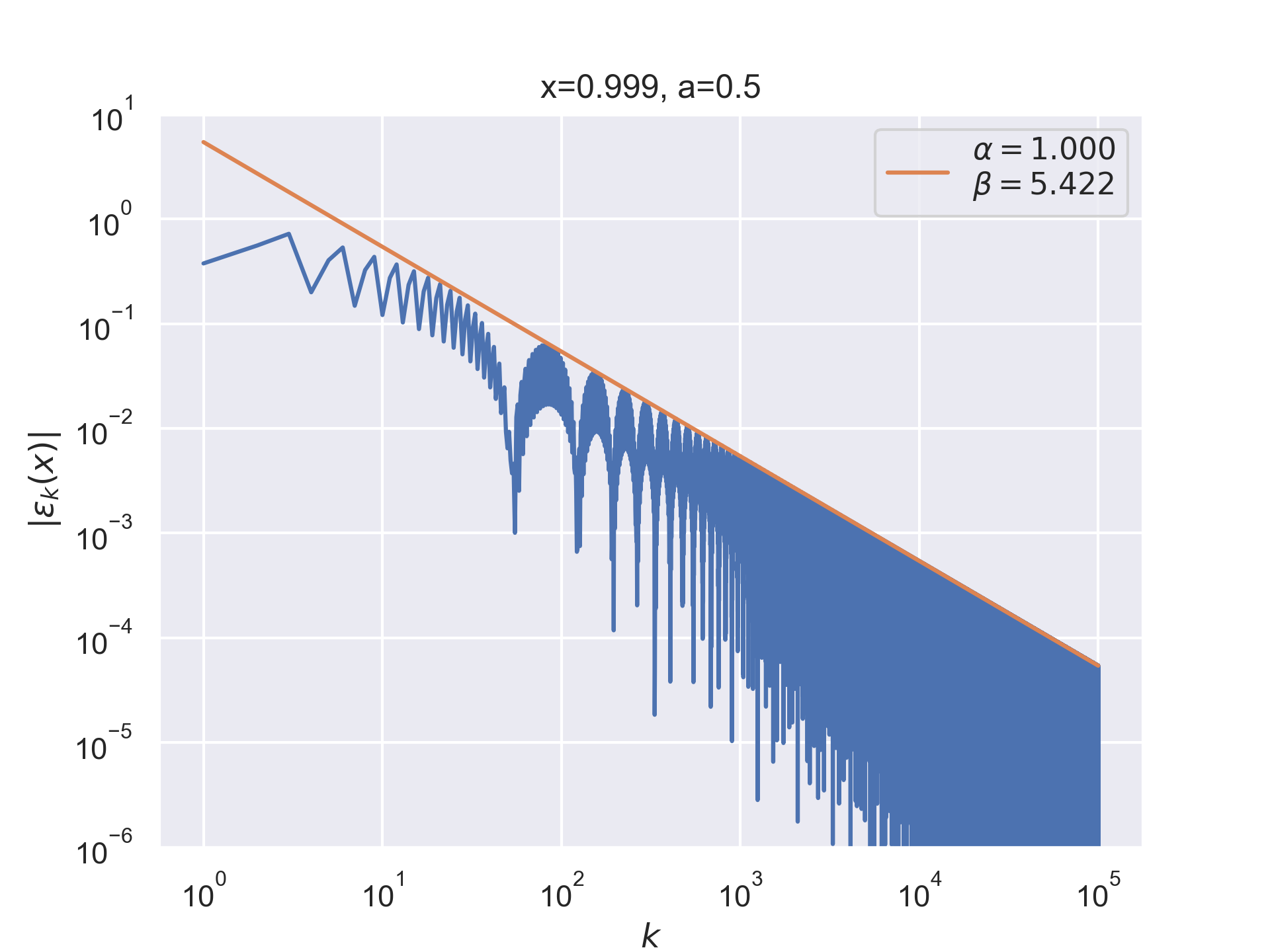
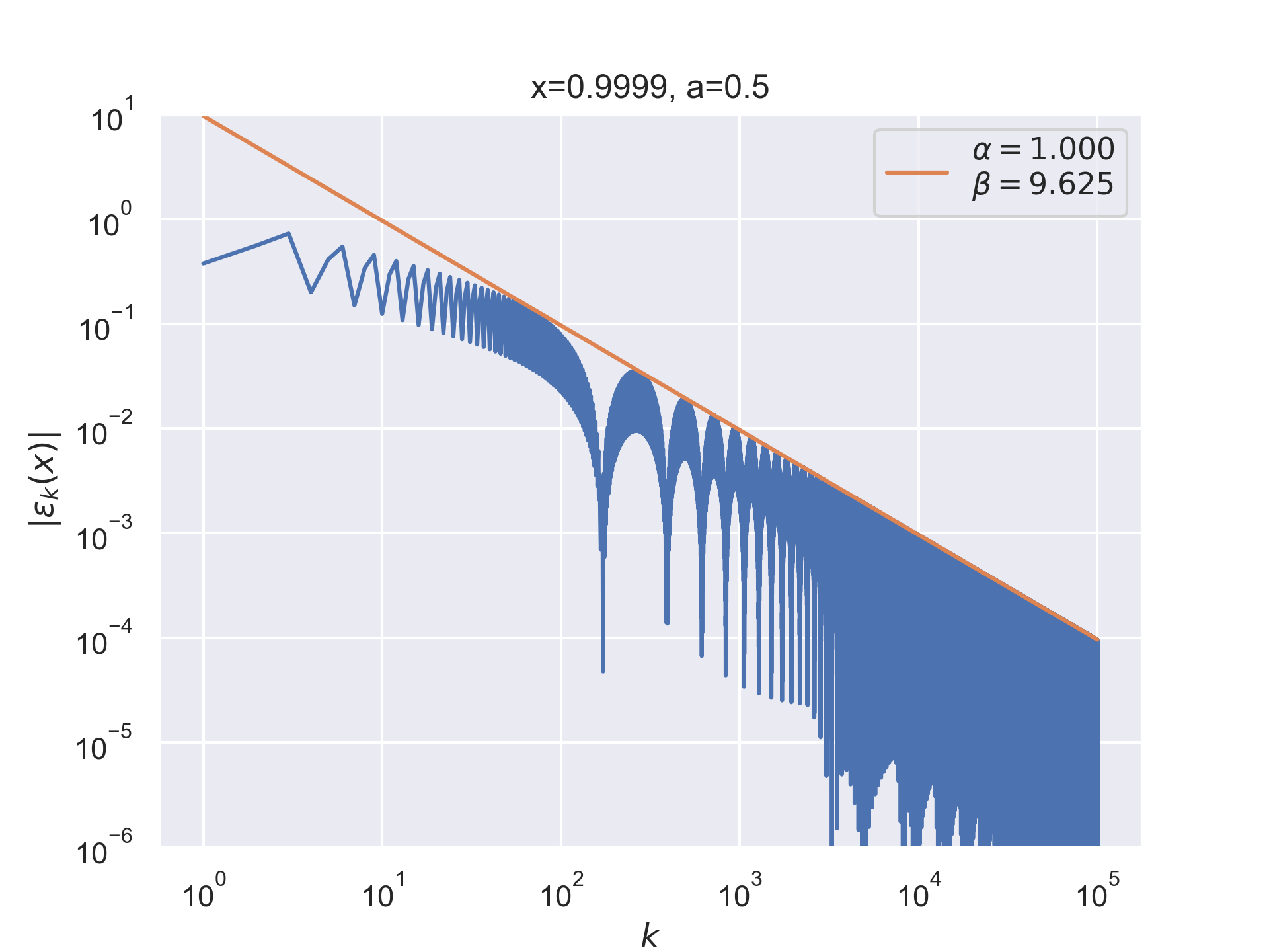
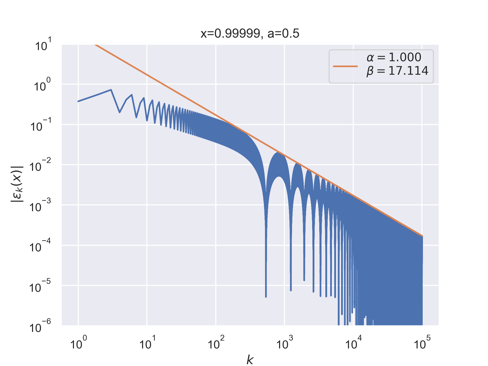
Pointwise convergence near edges $±(1-ξ)$ has a rate of convergence $α=1$ but similarly to points near singularity as $x$ moves closer to the edges the distance of convergence $β$ increases. Also, the pre-asymptotic region, i.e., a region with a different convergence rate, is visible.

We have plotted the convergence distances $β$ into a graph as a function of $x$. We can see the behavior at the near edges and near singularity. Values in these regions can be plotted on a logarithmic scale.
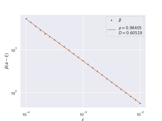

Near-singularity convergence distances $β(a±ξ)$ as a function of $x$ are linear at the logarithmic scale where the parameter $ρ≈1.0.$

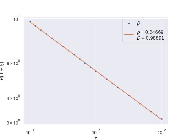
Near edges, convergence distances $β(±(1-ξ))$ as a function of $x$ are linear at the logarithmic scale where the parameter $ρ≈1/4.$
V Function
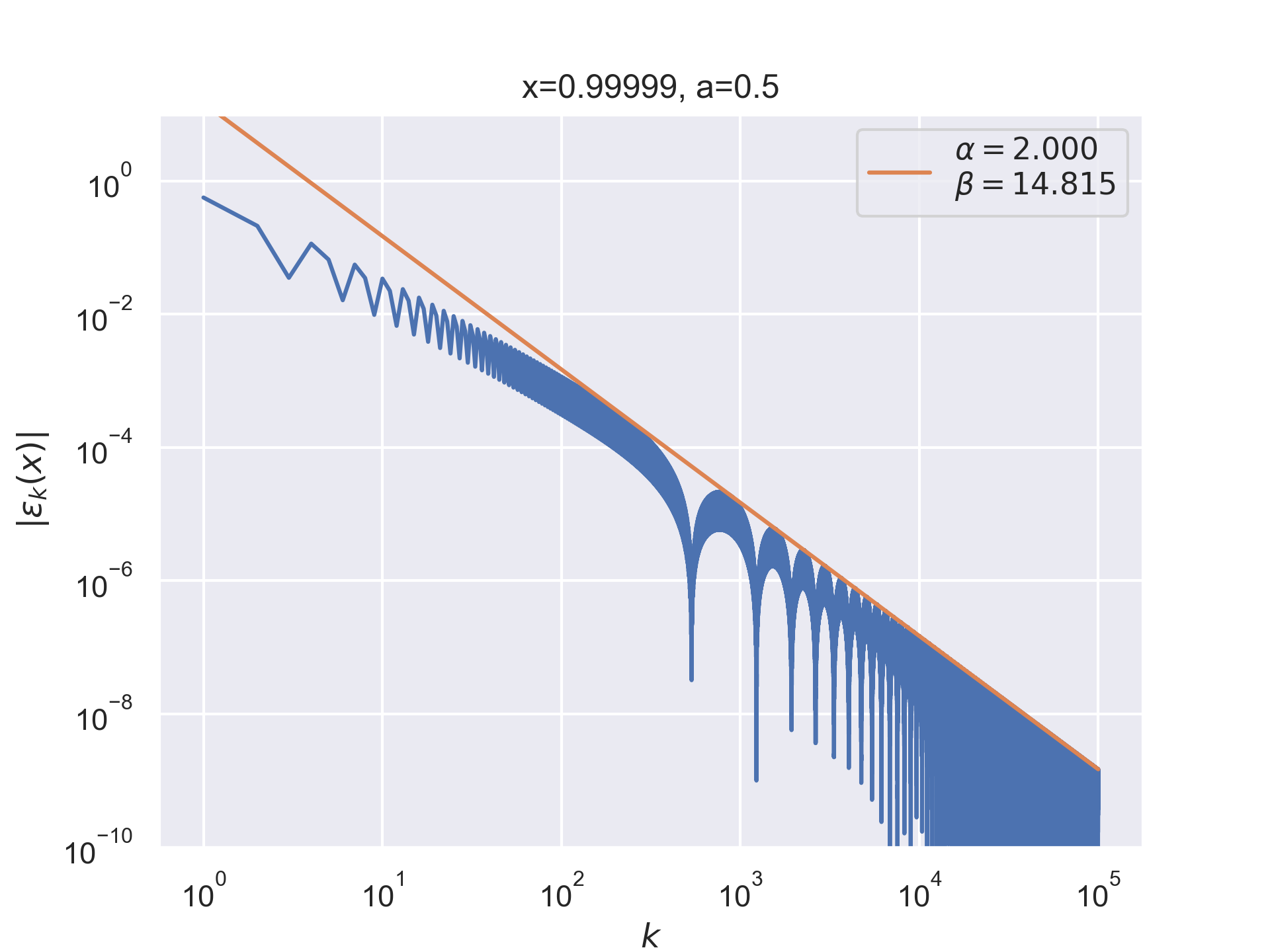
The following results where $a=0.5$ and $b=1$ for the V function. The results are similar, but not identical to those of the step function.


Pointwise convergence at the edges has a convergence rate of $α=1+1/2$.
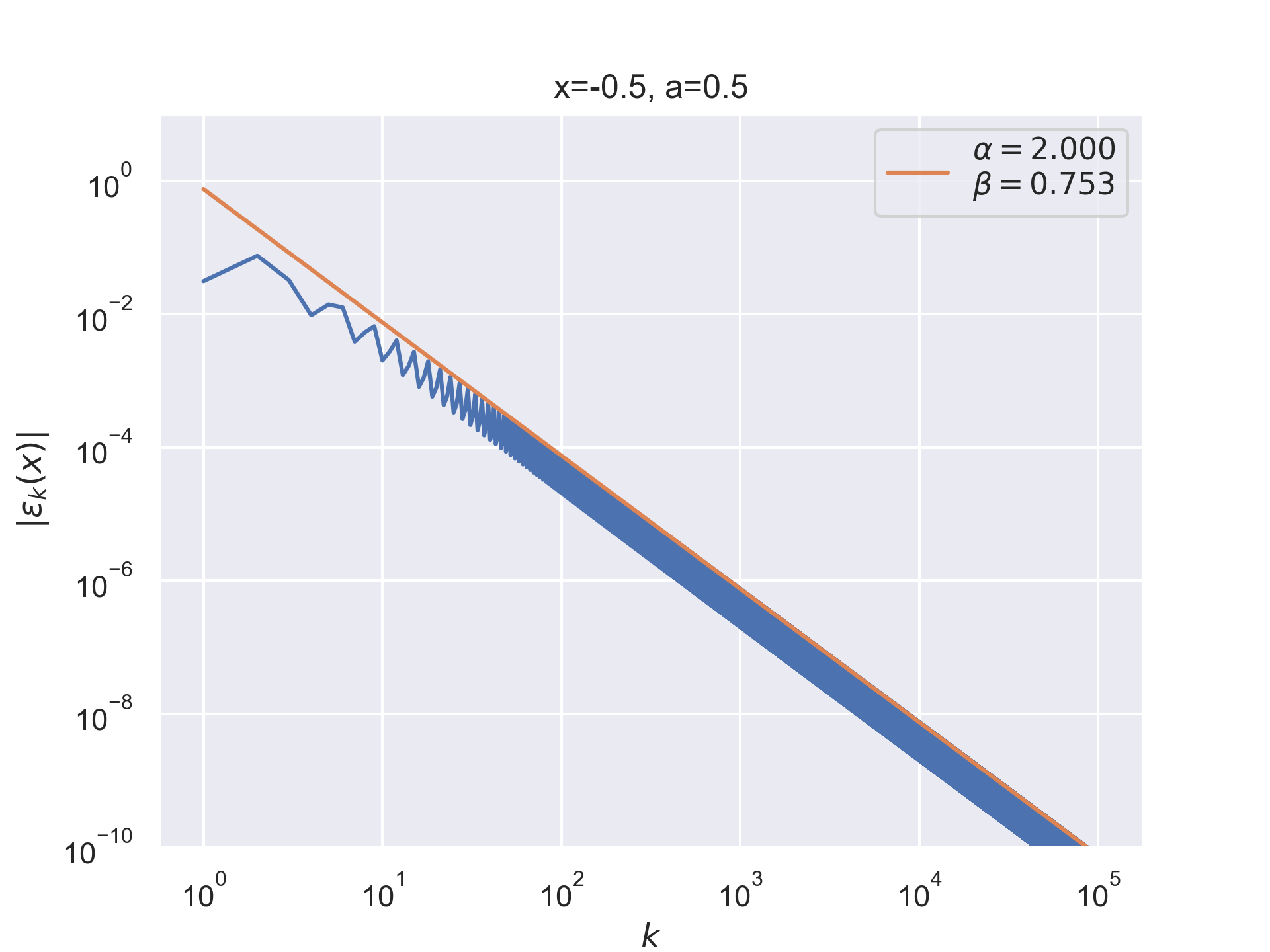

Pointwise convergence at the negation of singularity has convergence rate of $α=2$. Pointwise convergence at the singularity has a convergence rate of $α=1$. As can be seen, the convergence pattern is almost linear with very little oscillation.
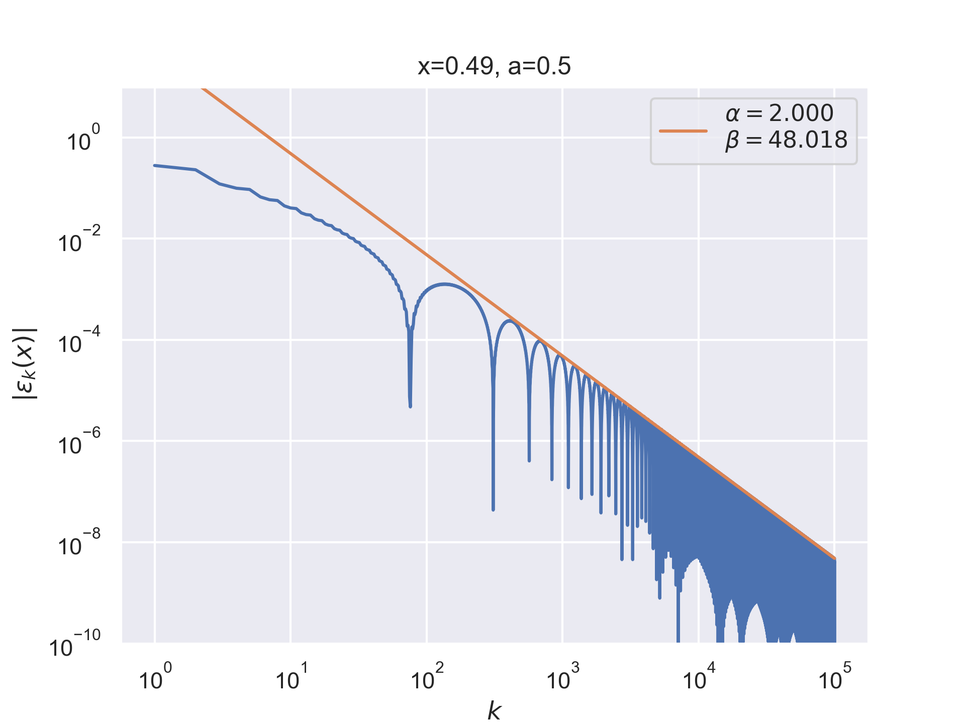
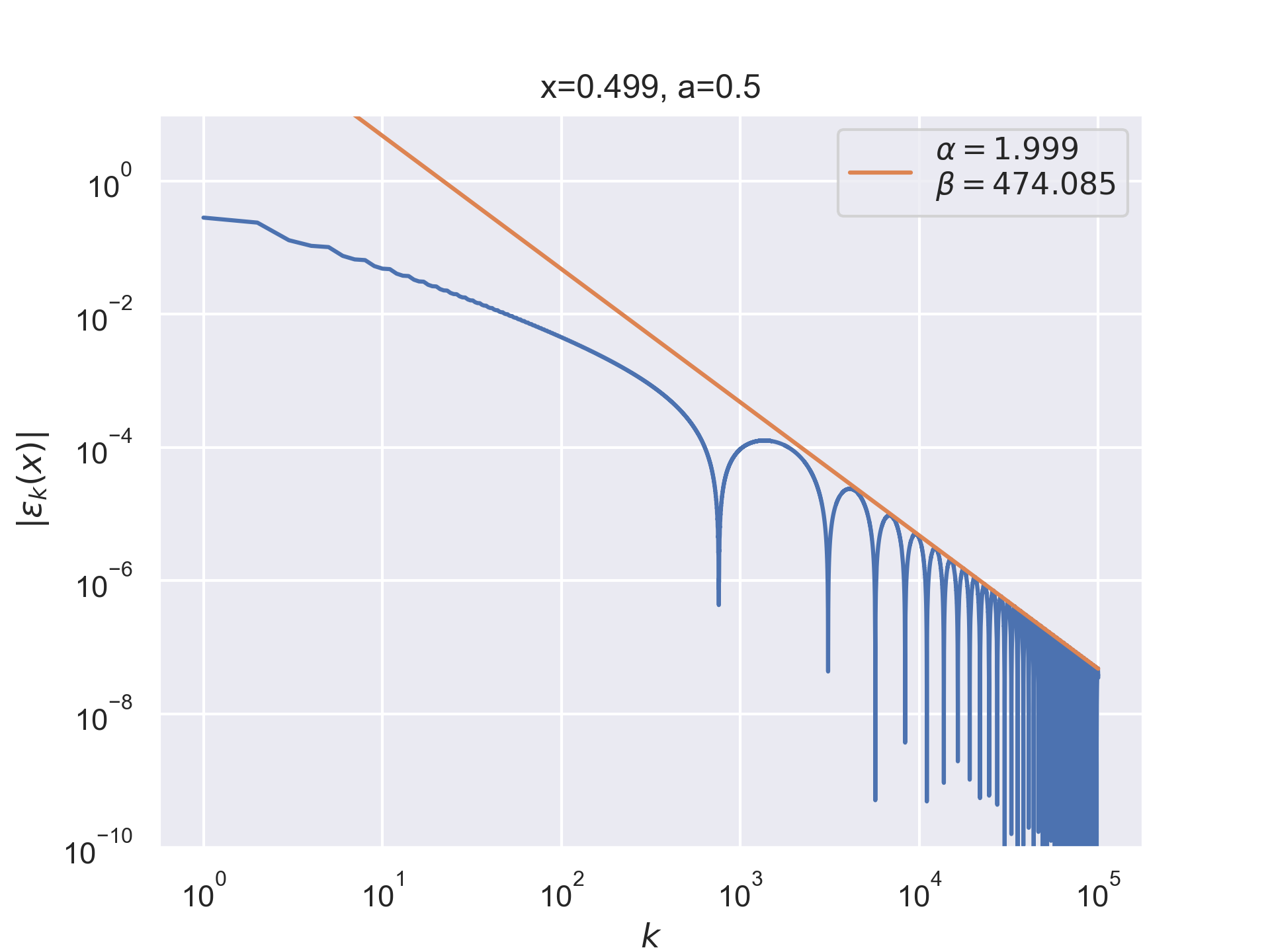


Pointwise convergence near singularity $a±ξ$ has a rate of convergence $α=2$, but as can be seen, the distance of convergence $β$ increases as $x$ moves closer to the singularity from either side.
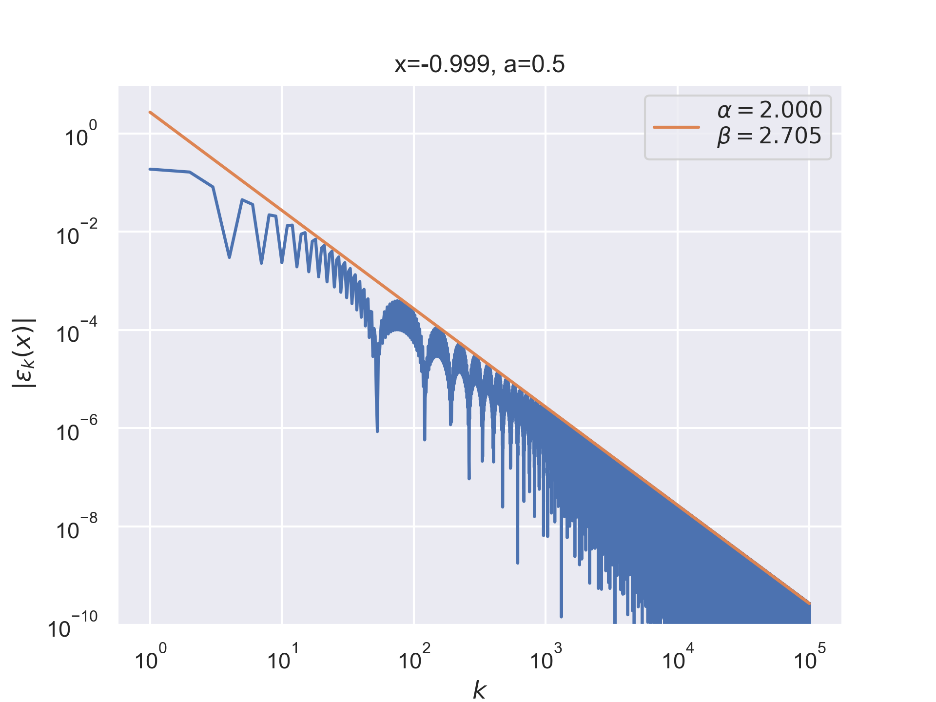
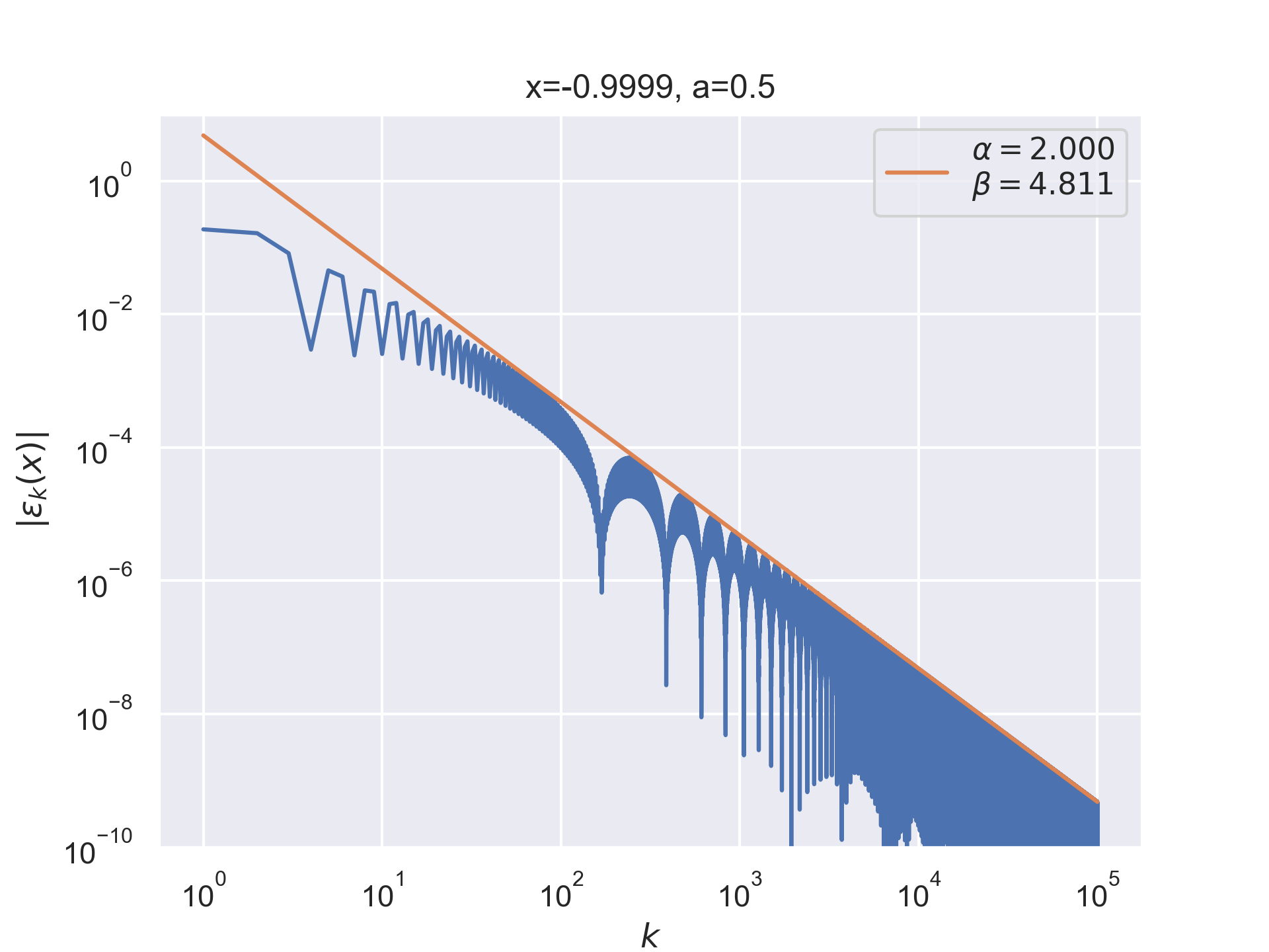
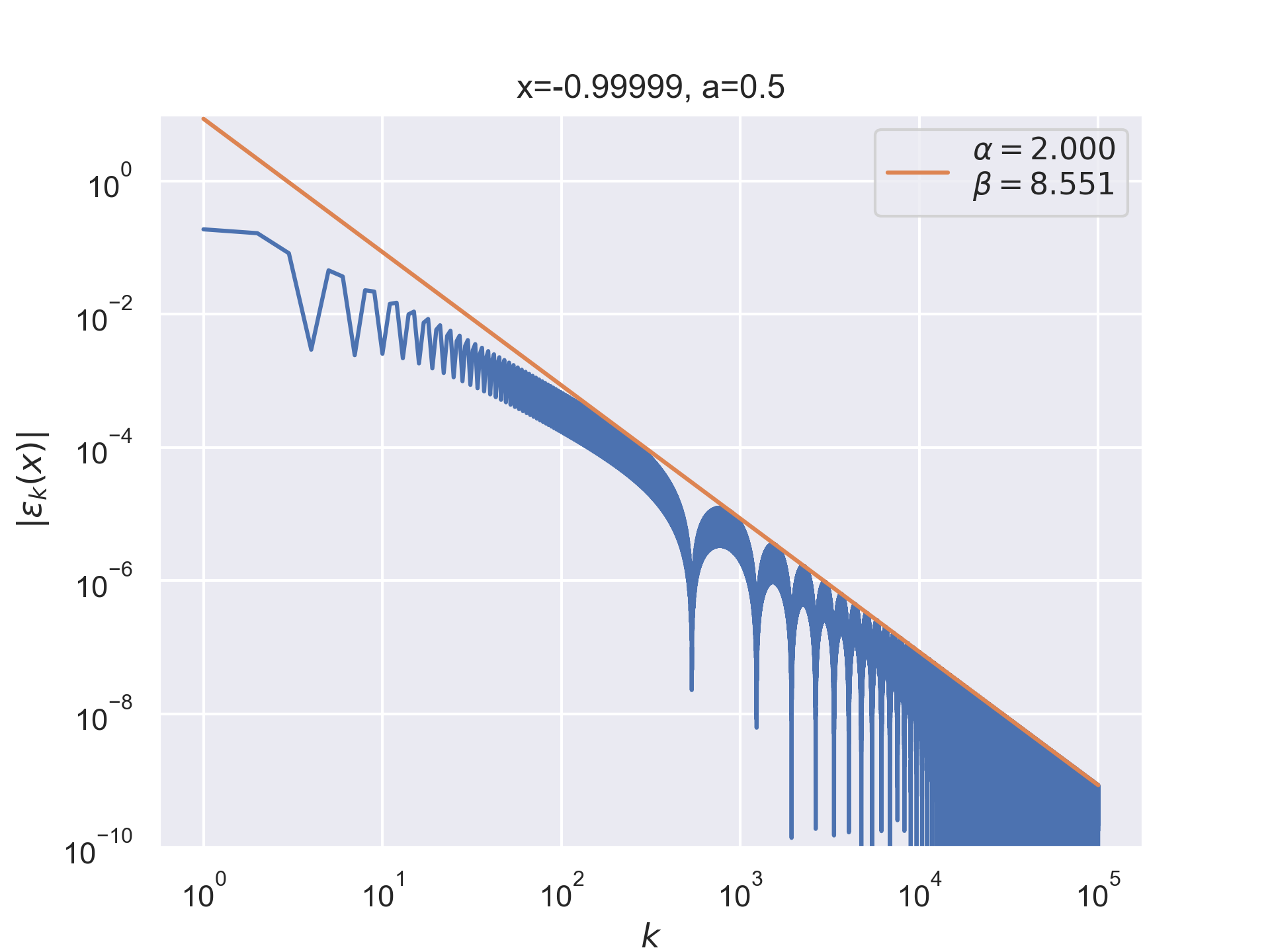
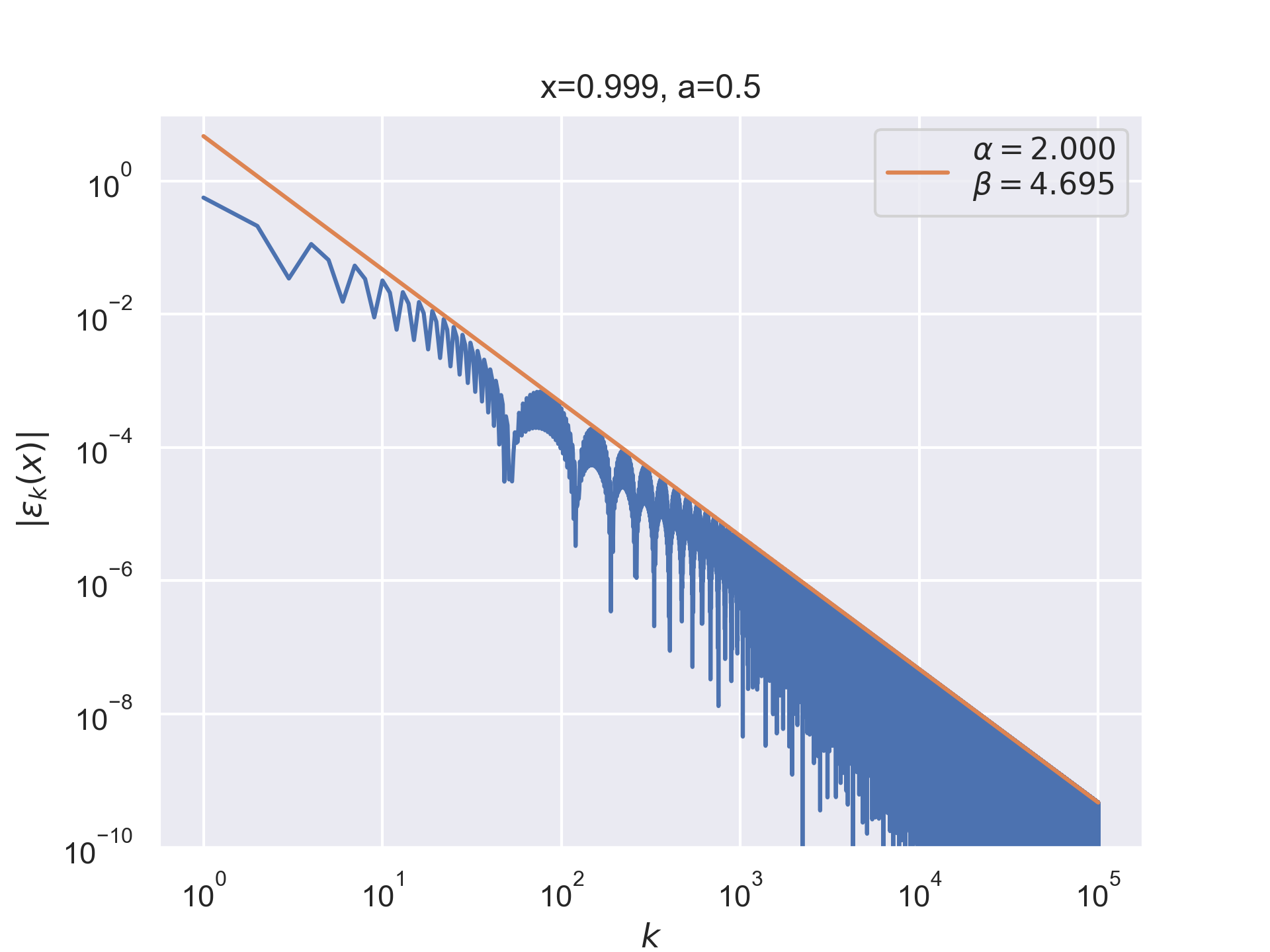
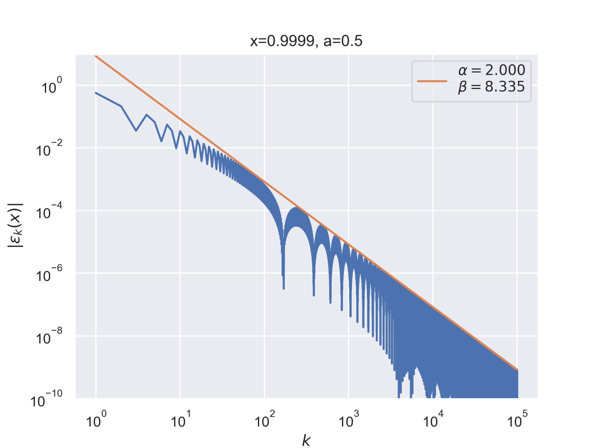
Pointwise convergence near edges $±(1-ξ)$ has a rate of convergence $α=2$ but similarly to points near singularity as $x$ moves closer to the edges the distance of convergence $β$ increases. Also, the pre-asymptotic region, i.e., a region with a different convergence rate, is visible.

We have plotted the convergence distances $β$ into a graph as a function of $x$. We can see the behavior at the near edges and near singularity. Values in these regions can be plotted on a logarithmic scale.
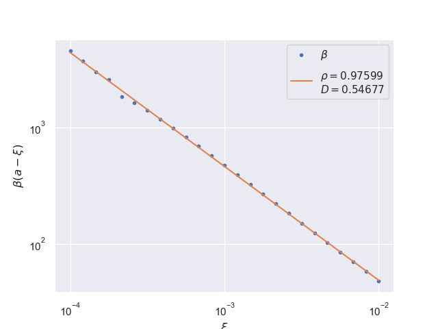

Near-singularity convergence distances $β(a±ξ)$ as a function of $x$ are linear at the logarithmic scale where the parameter $ρ≈1.0.$
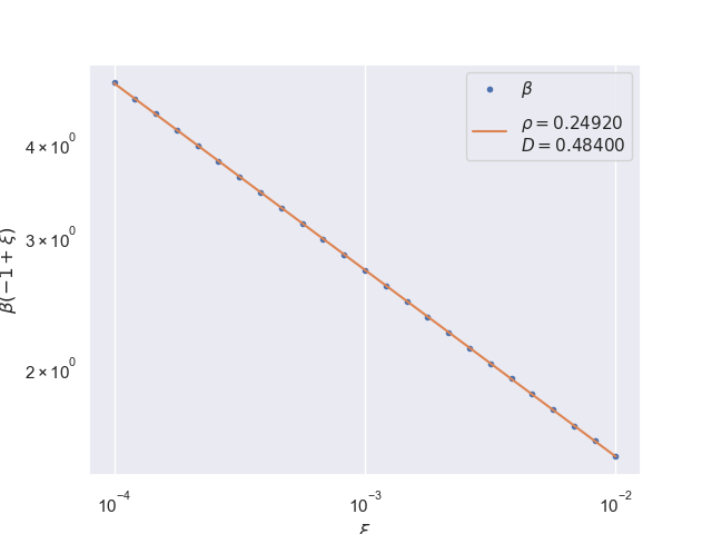

Near edges, convergence distances $β(±(1-ξ))$ as a function of $x$ are linear at the logarithmic scale where the parameter $ρ≈1/4.$
Conclusions
The results show that the Legendre series for piecewise analytic functions follows the conjectures $\eqref{convergence-rate}, \eqref{convergence-distance-near-singularity}$ and $\eqref{convergence-distance-near-edges}$ with high precision upto very high degree series expansion.
The future research could be extended to study the effects of the position of the singularity $a$ to the constant $D$ or to study series expansion using other classical orthogonal polynomials and special cases of Jacobi polynomials such as Chebyshev polynomials. However, their formulas are unlikely to have convenient closed-form solutions and could, therefore, be more challenging to study.
Contribute
If you enjoyed or found benefit from this article, it would help me share it with other people who might be interested. If you have feedback, questions, or ideas related to the article, you can contact me via email. For more content, you can follow me on YouTube or join my newsletter. Creating content takes time and effort, so consider supporting me with a one-time donation.
References
Babuška, I., & Hakula, H. (2014). On the $p$-version of FEM in one dimension: The known and unknown features, 1–25. Retrieved from http://arxiv.org/abs/1401.1483 ↩︎ ↩︎
Babuška, I., & Hakula, H. (2019). Pointwise error estimate of the Legendre expansion : The known and unknown features. Computer Methods in Applied Mechanics and Engineering, 345(339380), 748–773. https://doi.org/10.1016/j.cma.2018.11.017 ↩︎ ↩︎
Jaan Tollander de Balsch
Jaan Tollander de Balsch is a computational scientist with a background in computer science and applied mathematics.